Presented at IEEE Conference on Networking, Architecture, and Storage (NAS-2016):
Mathematics is the art of giving the same name to different things.
Henri Poincare
The question is: how to compute distribution of states of clustered nodes in a large distributed cluster running a steady workload? The cluster is fully distributed, and: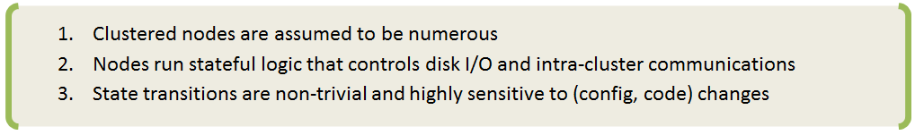 None of this is uncommon. For one thing, we live at a time of ever-exploding problem sizes. Bigger problems lead to bigger clusters with nodes that, when failed, get replaced wholesale.
And small stuff. For instance, eventually consistent storage is fairly common knowledge today. It is spreading fast, with clumps of apps (including venerable big data and NoSQL apps) growing and stacking on top.
Those software stacks enjoy minimal centralized processing (and often none at all), which causes CAP-imposed scalability limits to get crushed. This further leads to even bigger clusters, where nodes run complex stateful software, etcetera.
Why complex and stateful, by the way? The most generic sentiment is that the software must constantly evolve, and as it evolves its complexity and stateful-ness increases. Version (n+1) is always more complex and more stateful than the (n) – and if there are any exceptions that I’m not aware of, they only confirm the rule. Which fully applies to storage, especially due to the fact that this particular software must keep up with the avalanche of hardware changes. There’s a revolution going on. The SSD revolution is still in full swing and raging, with SCM revolution right around the corner. The result is millions of lines of code, and counting. It’s a mess.
It’s been noted before that Ceph benchmarks produce results that are lower than expected. Take for instance the most recent FAST’16 [BTrDB] paper (quote):
<snip> Applying this backpressure early prevents Ceph from reaching pathological latencies. Consider Figure 9a where it is apparent that not only does the Ceph operation latency increase with the number of concurrent write operations, but it develops a long fat tail, with the standard deviation exceeding the mean. Furthermore, this latency buys nothing, as Figure 9b shows that the aggregate bandwidth plateaus…
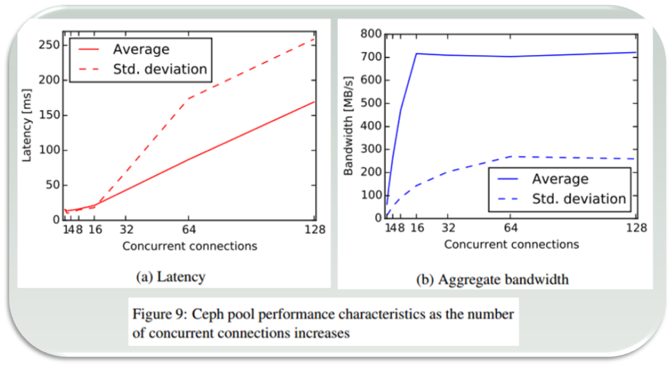
The above is indeed a textbook case (courtesy of [BTrBD]) of fat-tailed distribution, the one that deviates from its mean with high probability having either undefined or unbounded standard deviation (sigma). But wait.. the fat-tailed latency problem is by no means Ceph-specific.
Disclaimer:
Nexenta produces a competing solution that is called NexentaEdge. Secondly, needless to say that opinions expressed in this text are strictly and solely my own.
There are multiple reasons to single-out Ceph, the most researched and likely the most widely used general-purpose distributed storage stack. Ceph is an open source project as well, open for in-depth reviews. CRUSH remains one of the best content distribution algorithms. In sum, Ceph is as close as it gets to being a representative of the current generation – generation of post-Dynamo distributed storage systems.
The problem though affects majority of fully-distributed storage systems. To add insult to injury, it cannot be easily bug-fixed. The fat-tailed, heavy-tailed, long-tailed latency problem is in fact the other side of the uniformly-distributed “coin”.
A distributed storage cluster consists of multiple user-facing Storage Initiators (henceforth, “initiators”) and multiple reading/writing Storage Targets (“targets”).
Both initiators and targets execute concurrently and in parallel, the former – app requests, the latter – disk I/Os. Often {initiator + target} pairs are bundled as dual-function daemons within their respective clustered nodes – case in point (hyper)converged architectures, but not only.
The defining characteristic of a fully distributed cluster is that the path from an initiator to a target is direct. The datapath does not “cross” any central authority.
There is a lot of varying intelligence typically built into existing initiators, to help them decide where and how to route I/O requests. This intelligence, however, executes in the management and control (error processing) planes leaving fast path data distribution decisions totally up to the clustered frontend – to a given storage initiator.
This is exactly why do we have the following generic conflict – in Ceph, and in Swift, and in others.
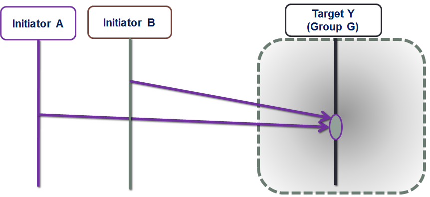
Figure 1. The Conflict
The figure depicts initiators A and B simultaneously reaching out to the same target Y. Since there’s no metadata server (MDS), centralized arbiter/load-balancer or any other kind of central logic in the datapath, each initiator simply goes ahead and reaches out based on the best information it had at the time.
From the target Y’s perspective, however, it just happened so that the two requests arrive in rapid succession within the same interval – the interval that, on average, corresponds to a single I/O request under a given workload (aka inter-arrival time).
Visualize a storage cluster consisting of identical nodes, where user data is uniformly distributed by multiple initiators, thus providing, on average, well-balanced resource utilization: CPU, network, I/O bandwidth and disk capacity of individual targets. Here’s the pertinent question: what is the probability of a conflict depicted above, where storage targets are forced to handle multiple requests within a single interval of time.
In statistics, a Poisson experiment must have the following defining properties:
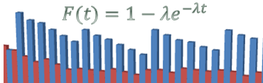
To make the connection, I’ll go out on a limb and say this: a very large fully distributed storage cluster under a fully random workload and sufficiently large working set can be (***) approximated as a massive Poisson experiment-generating machine. Whereby the target’s chances to see two or more I/O requests during a time interval t would compute as: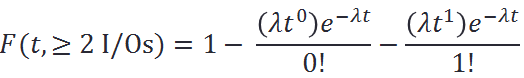 Therefore, at a sustained workload of, say, modest 10K per-target IOPS, the average inter-I/O interval would be 100μs. Given uniform distribution of I/O requests, the probability of two or more requests within this average 100μs interval is precisely:
![]() Meaning, for at least a quarter of all 100μs long intervals each target should expect to handle at least 2 interval-sharing requests. And in about 2% of all time the number spikes up to 4 or more, as per:
Meaning, for at least a quarter of all 100μs long intervals each target should expect to handle at least 2 interval-sharing requests. And in about 2% of all time the number spikes up to 4 or more, as per:![]()
Since storage clusters normally run many hours, days and months at a time, the 2% must be understood as accumulated minutes and hours of random 4x spikes.
Uniform distributions fair well when the cluster is – on average – underutilized. But if and when the load and pressure grows beyond 50% utilization and the resulting average per-I/O interval shrinks proportionally, then very quickly and quite frequently the targets are required to execute well above the average, and ultimately beyond their provisioned maximum bandwidth.
How frequently? At 50% utilization each clustered target must be expected to run at least 2 times faster than its own maximum performance at least 2% of the time. That is, assuming of course that the entire storage system can be modeled as a Poisson process.
But can it?
(***) Poisson processes are memoryless and, simultaneously, stateless – the two fine and abstract properties that are definitely not present in any real-life storage situation, distributed or local. Things get cached and journaled, aggregated and deduplicated. Generally, storage nodes (like the ones shown on Fig. 1) at any point in time have a wealth of accumulated state to deal with.
There are also multiple ways by which the targets may share their feedback and their own state with initiators, and each of these “ways” would create an additional state in the corresponding cluster-representing Markov’s chain which ultimately can become rather huge and unwieldy..
My sense though is (and here I’m frankly on shaky grounds) that given the (a, b, c, d) assumptions below, the Poisson approximation is valid and does hold.
(a) large fully distributed storage cluster;
(b) random workload;
(c) massive working set that tramples any and every attempt to cache;
(d) direct and uniform initiator ⇒ target distribution of data.
At the very least it gives an idea.
To recap:
The idea is to inject a bit of centralization into the otherwise fully and uniformly distributed cluster, to provide for scale and, simultaneously, true balance under stress. An example of one such protocol follows, along with benchmarks and comparison in the second (and separate) part of this text.
The implementation involves homegrown SURGE framework that is written in Go. I’m using Go mostly due to its built-in goroutines and channels – the language primitives that were invented to quickly write pieces of communicating logic that independently and concurrently run inside distributed “nodes”. As many nodes as your heart desires..
In SURGE each storage node (initiator or target) is a separate lightweight thread: a goroutine. The framework connects all configured nodes bi-directionally, via a pair of per node (Tx, Rx) Go channels. At model’s startup all clustered nodes (of this model) get automatically connected and ready to Go: send, receive and handle events and I/O requests from all other nodes.
There are various infrastructure classes (aka types) and utilities reused by the previously implemented models, for instance a rate bucket type that helps implement network and disk bandwidth limitations, and many more (see for instance the entry on this site titled Choosy Initiator).
Each SURGE model is an event-distributing event-driven machine. Quoting one previous text on this site:
Clustered configuration is practically unlimited. Each data frame and each control packet is a separate timed event over a separate peer-to-peer channel. The number of events exchanged during a single given benchmark is, frankly, mind-blowing – it blows my mind, it still does.
The new model (main piece of the source code here) represents a storage cluster that consists of load balancing groups of storage targets. Group size is configurable, with the only guideline that it corresponds to the required redundancy – due to the fact that each group acts as a whole as far as storing/retrieving redundant content.
The protocol leverages multicast replication of user data, and control plane that is, at least in part, terminated by a per-group selected leader, aka Group Proxy (from here on simply: proxy). In the simulation a proxy is a storage target with a minimal ID inside its own group.
Let’s see how it works without going yet into much detail – picture below illustrates the write/put sequence: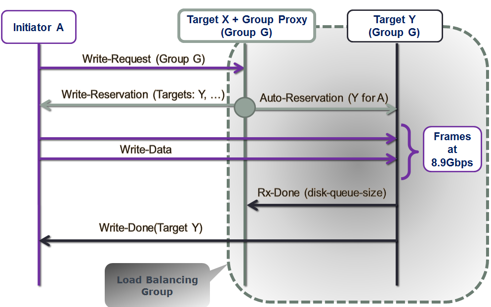
Figure 2. Write Sequence
As far as read/get, the pipeline starts with the read request delivered to all members of the group (Fig. 3). The idea is the same though: it is up to the proxy to decide who’s handling the read. More exactly: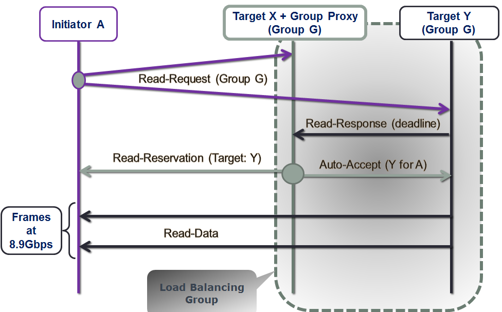
Figure 3. Read Sequence
Notice that in both read and write cases it is the group proxy that performs behind-the-scenes tracking of who-does-what-when for the entire group. The proxy, effectively, is listening on everything transpiring on the group-targeting control plane, and makes inline I/O routing decisions on behalf of the rest of group members.
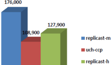
Wrapping up: one quick summary chart that shows the respective with group proxy and without group proxy benchmark-average performances expressed as chunks-per-second. The 50% read, 50% write workload is directed into 90 simulated targets by as many initiators, and the chunk sizes are 128K on the left, and 1M on the right, respectively:
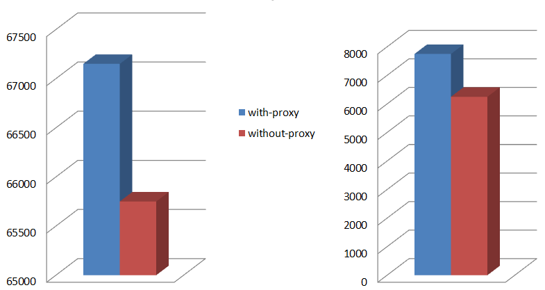
Figure 4. Average throughput
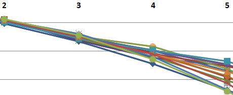
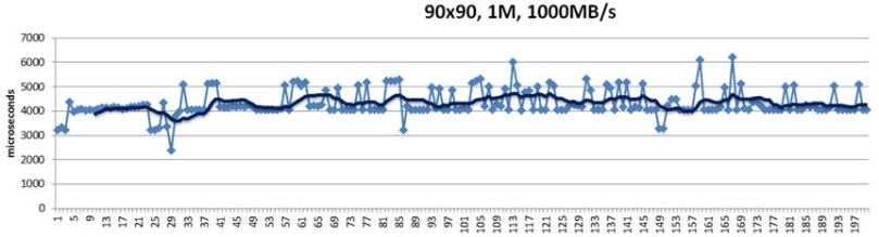
And here’s the throughput over time, for the same 50%/50% workload and 1MB chunk size:
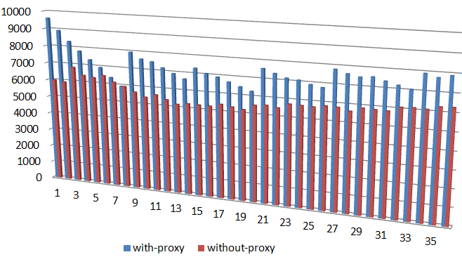
Figure 5. Throughput for 1M chunk
This experiment corresponds to the 1ae1388 commit. In the second upcoming part of the series I’ll try to show how exactly the comparison is done, and why exactly the results are what they are.
Evolution, some say, moves is spiraling circles and cycles. Software paradigms evolve and mutate, with every other iteration reintroducing stuff that was buried deep in the past. Or so it seems.
Post-Dynamo clusters that have evolved in forms of distributed block arrays, object storage clusters and NoSQL databases, reject any centralized processing in the datapath. There is a multifaceted set of interesting limitations that comes with that. What could be the better protocol? To be continued…
In a fully distributed storage cluster (FDSC), one possible design choice for a new storage protocol is resource reservation (RR). There are certain distinct challenges though, when working out an optimal RR schema. On the storage initiator side, one critical question that arises is whether to accept an RR response a.k.a. a bid from a given target for a given I/O request. Or, alternatively, try to renegotiate, in hopes of getting a better reservation.
The absolutely best reservation is, of course, the one that allows I/O in question to start immediately and execute at full throttle.
Hence, choosy initiator in the title, the storage initiator that grapples with the dilemma: go ahead and accept possibly suboptimal arrangement, or renegotiate. The latter inevitably comes with the risk to receive future reservations that are even more delayed.
To bet or not to bet, that is the question. To find out, I’ve used SURGE: a discrete open source event simulation framework written in Go (https://golang.org/doc/). The source includes a bunch of concrete protocol models (that run) and the usual README to get started.
OK, let’s do some definitions.
The three key aspects of a FDSC are self-containment, full connectivity, and hashed distribution:
Note separately that the letter ‘S’ in FDSC also reads as “symmetric”. In symmetric clusters, each node performs a dual role of storage initiator and storage target simultaneously.
For now let’s just say that large fully distributed clusters counting hundreds or thousands initiators and targets require a different intra-cluster transport. That’s #1, the point that maybe does not sound very controversial. To add controversy (just for the heck of it), here’s the point #2: for large and super-large FDSC it makes a lot of sense to use RR based transport protocols. One of the key proof points boils down to convergence.
Convergence time is the time it takes for existing link-sharing (path-sharing) flows to converge on their respective optimal rates when a new flow is being added or an existing flow removed. All things being equal, each of the N flows eventually must take 1/Nth of the total bandwidth.
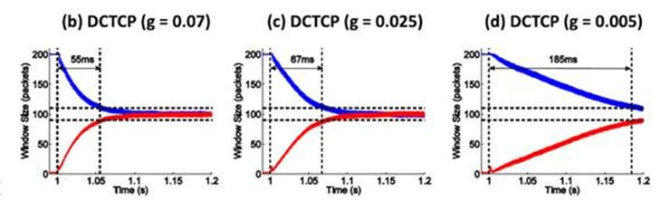
Figure 12 in the research paper at http://goo.gl/JUlijH shows DCTCP convergence times.
Red flow (below) is added after the blue flow has reached its steady and close-to-optimal state. The research estimates DCTCP convergence times on a 10GE network ranging anywhere from 229*d to 770*d, where d is the propagation delay. This is a considerable time corresponding to several fully transferred 128K payloads even for a very favorable (as far as speedy convergence) value of d in the order of few microseconds.
In presence of multiple flows the picture gets substantially more messy but the bigger point is: irrespective of the particular link-sharing transport, during the time N flows are converging from (N-1) or (N+1), they all execute at sub-optimal rates resulting in overall sub-optimal network utilization. Hence, an appeal of the RR approach: eliminate resource sharing. Utilization time slots are simply negotiated. There will be no unexpected start-IO, complete-IO, and add-flow, delete-flow events in the middle.
If there exists anything similar in real life, that could be a timeshare ownership. On the networking side examples include RSVP in its unicast and multicast realizations (RFC2205).
In all cases (including timeshare) and independently of the concrete resource reservation protocol, each successful RR negotiation comes with a time window in combination with a full set of requested targets resources – for exclusive usage (during a given time window) by a given pending request (emphasis on exclusive). For each I/O request, there is a natural progression:
I/O request =>
   potential targets =>
      RR negotiation(s) =>
          data flows to/from ...
This results in network flows executing as prescribed by non-overlapping time windows granted in turn by the respective selected targets.
The figure below shows one possible “resource reservation, renegotiated” (RRR) scenario:
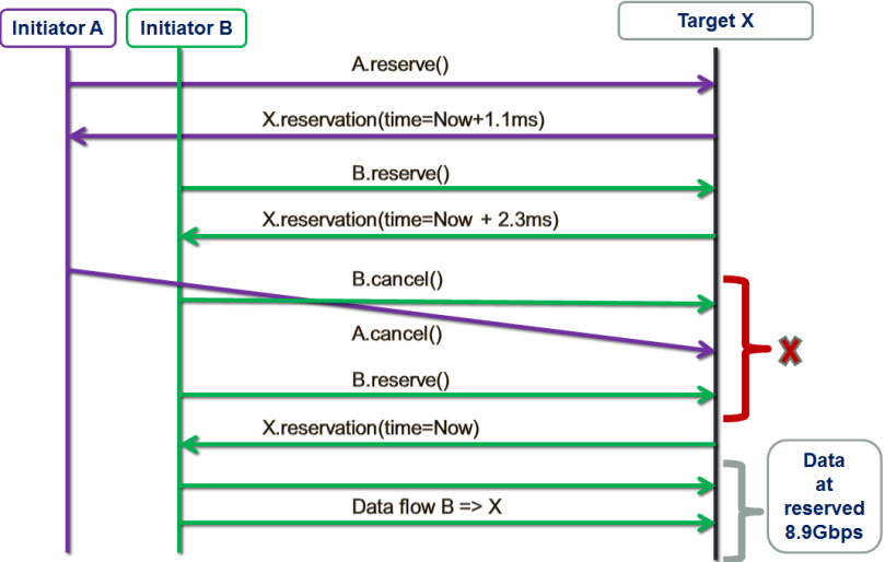
There are two storage initiators: purple A and green B. The initiators are trying to establish data flows with the same target X at approximately the same time.
First, initiator A tentatively reserves target X for a window starting 1.1ms later (from now), which roughly corresponds to the time target X needs to complete a (presumably) already queued 1MB transaction (not shown here).
Next, initiator B tentatively reserves X for the adjacent X’s time window at 2.3ms from now. Red X on the picture indicates the decision point.
In this example, instead of accepting whatever is presented to it at the moment, B decides that 2.3ms is too much of a delay and cancels. Simultaneously, A cancels as well, possibly because it has obtained more attractive bids from other storage targets that are not shown here. This further results in B getting the optimal reservation and utilizing it right away.
The idea that at least sometimes it does make sense to take a risk and renegotiate requires proof. Fortunately, with SURGE we can run massive simulations to find out.
Replicast is a one FDSC-friendly RR-based protocol that was previously described – see for instance SNIA presentation Beyond Consistent Hashing and TCP.
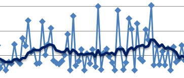
Replicast-H (where H stands for hybrid) entails multicast control plane and unicast data. Recall that RR negotiation is a part of the reservations-based protocol control plane. When running a hybrid version of the Replicast, we negotiate up to (typically) 3 successive time windows to perform a write. We then often see the following picture:
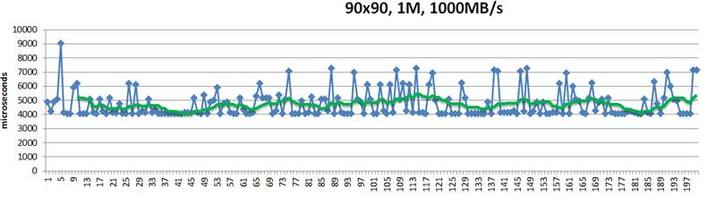
This above is a 200-point random sample that details latencies of 1MB size chunks written into their hashed target destinations. Green trendline in the middle shows 10-point moving average. This is a “plain” Replicast-H benchmark where each target’s bid is taken at a face value and never renegotiated.
The cluster in this case combines 90 targets and 90 storage initiators with targets operating at 1000MB/s disk throughput. Finally, there is a non-blocking no-drop 10Gbps that connects each target with each initiator.
In the simulation above 10% of the bandwidth is statically allocated for control traffic. With 1% accounting for network headers and miscellaneous overhead, that leaves 8.9Gbps for (pure) data.
In the idealistic conditions when a given initiator does not have any competition from others, the times to execute a 1MB write to a single target would be, precisely:
Given 3 copies, the request could (ideally) be fully executed in slightly more than 4 milliseconds, including control handshakes and acknowledgements.
There is, however, inevitably a competition resulting in reservation conflicts and delays, and further manifesting itself in occasional end-to-end spikes up to 7ms latency and beyond – see the picture above.
In depth analysis of traces (that I will skip here) indicates that, indeed, one possible reason for the spikes is that initiators accept reservations too early. For instance, the initiator that executed the #5 in the sample (Fig. 3) could likely do better.
This “with renegotiation” flavor of the protocol adds a new configuration variable that currently defaults to 3 times RTT on the control plane:

Note: to go directly to the github source, click this and other similar code fragments. At runtime, this model will double the wait time and renegotiate reservations if and when the actual waiting time (denoted as ‘idletime’ below) exceeds the current value:
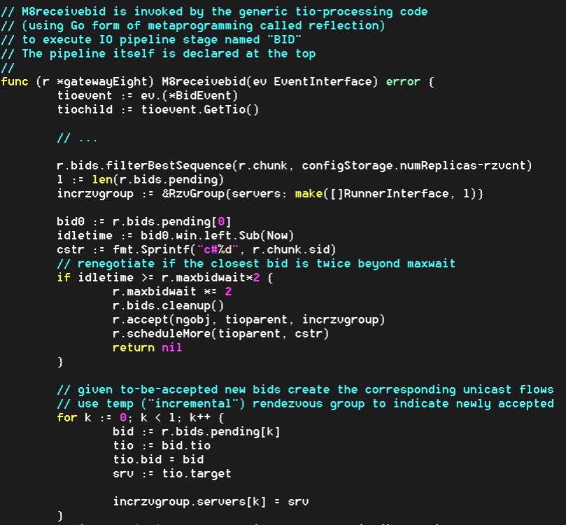
In addition, since 3 times RTT is just a crude initial guess, each modeled gateway (a.k.a. storage initiator) recomputes its value (‘r.maxbidwait’ in the code) for the next write request, averaging the previous value and the current one:

What happens after the first few transactions is that each initiator independently computes an objective average delay and from there on renegotiates only when the newly collected reservations collectively result in substantially bigger delay (in other words, the initiator renegotiates only when it “thinks” it could get a better deal).
Here’s the SURGE-simulated result for apples-to-apples identical configuration that runs 90 storage initiators and 90 storage targets, etc.:
Notice that there are no 7ms spikes anymore. They are simply gone.
For differently sized chunks and disk/backend throughputs, the average improvement ranges from 8% to 20%:
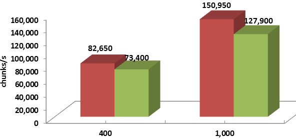
Legend-wise, red columns depict the “with renegotiation” version.
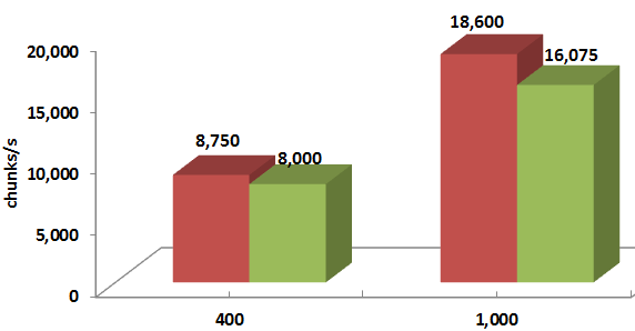
Thus, taking a risk does seem to pay off: RR based protocol where storage initiators are “choosy” and at least sometimes renegotiate their reservations outperforms its prior version.
As far as distributed system and storage software, finding out how it'll perform at scale - is hard.
Expensive and time-consuming as well, often impossible. When there are the first bits to run, then there’s maybe one, two hypervisors at best (more likely one though). That’s a start.
Early stages have their own exhilarating freshness. Survival is what matters then, what matters always. Questions in re hypothetical performance at 10x scales sound far-fetched, almost superficial. Answers are readily produced – in flashy powerpoints. The risk however remains, carved deep into the growing codebase, deeper inside the birthmarks of the original conception. Risk that the stuff we’ll spend next two, three years to stabilize will not perform.
The goal is modeling the performance of a distributed system of any size (emphasis on modeling, performance and any size). Which means – uncovering the behavioral patterns (periodic spike-downs and, generally, any types of pseudo-regular irregularities), charting throughputs and latencies and their respective distributions concealed behind performance averages. And tails of those distributions, those that are in the single-digit percentile ranges.
Average throughput, average IOPS, average utilization, average-anything is not enough – we need to see what is really going on. For any scale, any configuration, any ratios of: clients and clustered nodes, network bandwidth and disk throughput, chunk/block sizes, you name it.
Enter SURGE, discrete event simulation framework written in Go and posted on GitHub. SURGE translates (admittedly, with a certain effort) as Simulator for Unsolicited and Reservation Group based and Edge-driven distributed systems. Take it or leave it (I just like the name).
Go aka golang, on the other hand, is a programming language1 2.
Go is an open source programming language introduced in 2007 by Rob Pike et al. (Google). It is a compiled, statically typed language in the tradition of C with garbage collection, runtime reflection and CSP-style concurrent programming.
CSP stands for Communicating Sequential Processes, a formal language, or more exactly, a notation that allows to formally specify interactions between concurrent processes. CSP has a history of impacting designs of programming languages.
Runtime reflection is the capability to examine and modify the program’s own structure and behavior at runtime.
Go’s reflection appears to be very handy when it comes to supporting IO pipeline abstractions, for example. But more about that later. As far as concurrency, Rob Pike’s presentation is brief and to the point imho. To demonstrate the powers (and get the taste), let’s look at a couple lines of code:
In this case, notation 'go function-name' causes the named function to run in a separate goroutine – a lightweight thread and, simultaneously, a built-in language primitive.
Go runtime scheduler multiplexes potentially hundreds of thousands of goroutines onto underlying OS threads.
The example above creates a bidirectional channel called messages (think of it as a typed Unix pipe) and spawns two concurrent goroutines: send() and recv(). The latter run, possibly on different processor cores, and use the channel messages to communicate. The sender sends random ASCII codes on the channel, the receiver prints them upon reception. When 10 seconds are up, the main goroutine (the one that runs main()) closes the channel and exits, thus closing the child goroutines as well.
Although minimal and simplified, this example tries to indicate that one can maybe use Go to build an event-distributing, event-driven system with an arbitrary number of any-to-any interconnected and concurrently communicating players (aka actors). The system where each autonomous player would be running its own compartmentalized piece of event handling logic.
Hold on to this visual. In the next section: the meaning of Time.
In SURGE every node of a modeled cluster runs in a separate goroutine. When things run in parallel there is generally a need to go extra length to synchronize and sequence them. In physical world the sequencing, at least in part, is done for us by the laws of physics. Node A sending message to remote node B can rest assured that it will not see the response from node B prior to this sent message being actually delivered, received, processed, response created, and in turn delivered to A.
The corresponding interval of time depends on the network bandwidth, rate of the A ⇔ B flow at the time, size of the aforementioned message, and a few other utterly material factors.
That’s in the physical world. Simulated clusters and distributed models cannot rely on natural sequencing of events. With no sequencing there is no progression of time. With no progression there is no Time at all – unless…
Unless we model it. For starters let’s recall an age-old wisdom: time is not continuous (as well as, reportedly, space). Time rather is a sequence of discrete NOWs: one indivisible tick (of time) at a time. Per quantum physics the smallest time unit could be the Planck time ≈5.39*10-44s although nobody knows for sure. In modeling, however, one can reasonably ascertain that there is a total uneventful void, literally nothing between NOW and NOW + 1.
In SURGE, the smallest indivisible tick of time is 1 nanosecond, a configurable default.
In a running operating physical cluster each NOW instant is filled with events: messages ready to be sent, messages ready to be received, events being handled right NOW. There are also en route messages and events sitting in disk and network queues and waiting for their respective future NOWs.
Let’s for instance imagine that node A is precisely NOW ready to transmit a 8KB packet to node B:
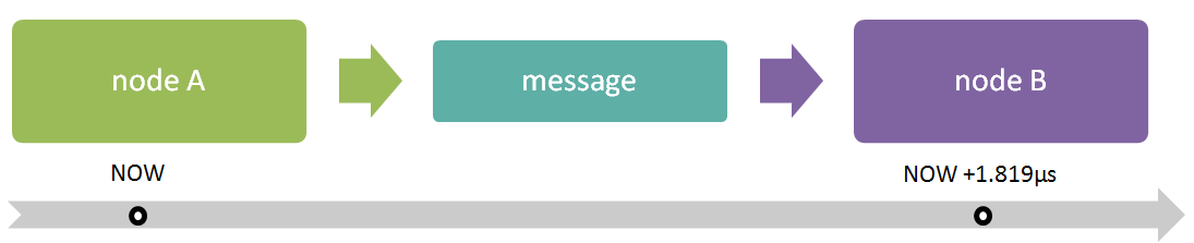
Given full 10Gbps of unimpeded bandwidth between A and B and the trip time, say, 1µs, we can then with a high level of accuracy predict that B will receive this packet (819ns + 1µs) later, that is at NOW+1.819µs as per the following:
In this snippet of modifiable-and-runnable code, the local variable sizebits holds the number of bits to send or receive while bwbitss is a link bandwidth, in bits per second.
Here’s a statement of correctness that, on the face of it, may sound trivial. At any point in time all past events executed in a given model are either already fully handled and done or are being processed right now.
A past event is of course an event scheduled to trigger (to happen) in the past: at (NOW-1) or earlier. This statement above in a round-about way defines the ticking living time:
At any instant of time all past events did already trigger.
And the collateral:
Simulated distributed system transitions from (NOW-1) to NOW if and only when absolutely all past events in the system did happen.
Notice that so far this is all about the past – the modeled before. The after is easier to grasp:
For each instant of time all future events in the model are not yet handled - they are effectively invisible as far as designated future handlers.
In other words, everything that happens in a modeled world is a result of prior events, and the result of everything-that-happens is: new events. Event timings define the progression of Time itself. The Time in turn is a categorical imperative – a binding constraint (as per the true statements above) on all events in the model at all times, and therefore on all event-producing, event-handling active players – the players that execute their own code autonomously and in parallel.
To recap. Distributed cluster is a bunch of interconnected nodes (it always is). Each node is an active Go player in the sense that it runs its own typed logic in its own personal goroutine. Nodes continuously generate events, assign them their respective computed times-to-trigger and fan them out onto respective Go channels. Nodes also continuously handle events when the time is right.
By way of a sneak peek preview of timed events and event-driven times, here’s a life of a chunk (a block of object’s data or metadata) in one of the SURGE’s models:
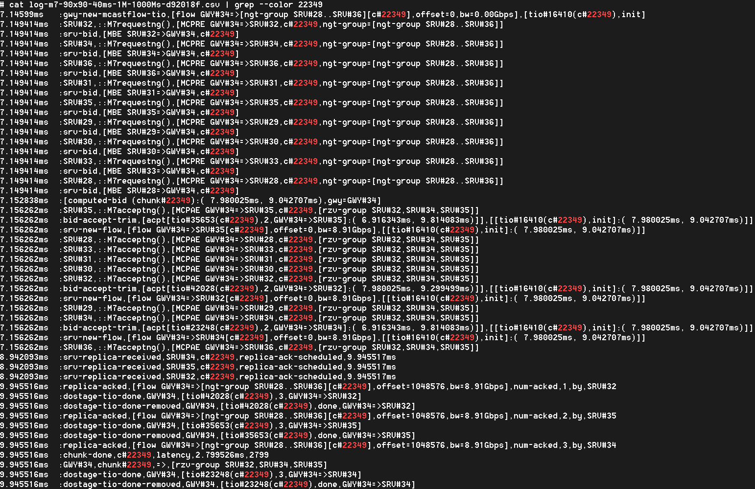
The time above runs on the left, event names are abbreviated and capitalized (e.g. MCPRE). With hundreds and thousands of very chatty nodes in the model, logs like this one become really crowded really fast.
In SURGE framework each and every event is timed, and each timed event implements the following abstract interface:
type EventInterface interface {
    GetSource() RunnerInterface
    GetCreationTime() time.Time
    GetTriggerTime() time.Time
    GetTarget() RunnerInterface
    GetTio() *Tio
    GetGroup() GroupInterface
    GetSize() int
    IsMcast() bool
    GetTioStage() string
    String() string
}
This reads as follows. There is always an event source, event creation time and event trigger time. Some events have a single remote target, others are targeting a group (of targets). Event’s source and event’s target(s) are in turn clustered nodes themselves that implement (RunnerInterface).
All events are delivered to their respective targets at prescribed time, as per the GetTriggerTime() event’s accessor. The Time-defining imperative (above) is enforced with each and every tick of time.
In the next installment of SURGE series: ping-pong model, rate bucket abstraction, IO pipeline and more.
