Mathematics is the art of giving the same name to different things.

Henri Poincare

1. Life’s most persistent question

The question is: how to compute distribution of states of clustered nodes in a large distributed cluster running a steady workload? The cluster is fully distributed, and:None of this is uncommon. For one thing, we live at a time of ever-exploding problem sizes. Bigger problems lead to bigger clusters with nodes that, when failed, get replaced wholesale.

And small stuff. For instance, eventually consistent storage is fairly common knowledge today.  It is spreading fast, with clumps of apps (including venerable big data and NoSQL apps) growing and stacking on top.

Those software stacks enjoy minimal centralized processing (and often none at all), which causes CAP-imposed scalability limits to get crushed. This further leads to even bigger clusters, where nodes run complex stateful software, etcetera.

Why complex and stateful, by the way? The most generic sentiment is that the software must constantly evolve, and as it evolves its complexity and stateful-ness increases. Version (n+1) is always more complex and more stateful than the (n) – and if there are any exceptions that I’m not aware of, they only confirm the rule. Which fully applies to storage, especially due to the fact that this particular software must keep up with the avalanche of hardware changes. There’s a revolution going on. The SSD revolution is still in full swing and raging, with SCM revolution right around the corner. The result is millions of lines of code, and counting. It’s a mess.

2. Queueing theory won’t help

The question therefore is, what’s really happening deep inside those clusters when they run steady? What is the big picture, the system-level view, the distribution of node states? Would it be possible to compute state-distributing PMFs or, at least, probability of their distributions?

One thing we know is that the cluster can be looked at as one humongous (I/O request in, I/O request out) queueing machine. Queueing machines belong to the Queueing Theory (QT) – a special kind of math that deals with waiting lines and random service requests.

In QT’s parlance the cluster is multi-server queueing model where I/O requests arrive and get serviced at certain rates. Or, alternatively, the model where I/O birth and death (completion) is happening at not yet identified probability distributions. Arrival rates and service times, the first and second moment of the above and their probability distribution, the birth-and-death – those are the QT’s abstractions that must be nailed to make any progress (with QT).

Queueing models, those that are fully researched and those that are not yet, are typically classified using standard Kendall’s notation A/S/c/* where the first three tokens stand for: A – arrival process, S – service time, c – number of servers. Much of the QT is devoted to M/M/* queues where both arrivals and service times are Markovian, that is, Poisson, that is memoryless. The most advanced and modern part of QT tries to deal with M/G/* and G/M/* models, where the ‘M’, again, stands for Markovian aka memoryless, and the G – general distribution.

Back to the question of whether QT is applicable. On one hand, it’ll be difficult to come up with anything less memoryless than a storage stack where state transitions are always based on the past and where the logic is constantly looking at what’d happened before, I/O-wise, how fast it had happened, and how optimal are the interim results.

Because, for instance, if it had happened fast we can extrapolate and say “ok, at this rate we are going to hit the wall soon, time to act now”. Or if, on the other hand, intermediate results (of aggregation, compression, deduplication) are below the expectation then again – we know it’s time to move the I/O along the chain.

Which is why on the level of any given server ensuing fluctuations are significant, albeit not significant enough to shake the entire large cluster out of its comfortable steady-state equilibrium. Those ripples are absorbed by the cluster. In the models I’m looking at right now those ripples are absorbed better if the cluster is larger..

However. Reliance/dependence on the memoryless-ness is not the biggest QT’s limitation, maybe not a limitation at all. After all, nobody says that a complex-but-deterministic logic will not manifest itself in some well-rounded probability distributions. Complex “black boxes” do produce simple distributions..

Yes, QT requires us to make assumptions with regards to distribution of I/O arrivals and completions, and state transitions in-between. And yes, QT prefers that those distributions are either fixed-probability, or binomial, or  exponential, Markovian, memoryless. But the way I see it, the real problem is that QT effectively asks us to use a “microscope” and focus it on one clustered node. The idea is, if you know exactly how a single server behaves, you can then model N servers and compute the distribution of node states.

But that’s exactly the wrong thing, for at least three different reasons:

• Reason #1: the servers do interact with each other, I/O wise, quite a bit. In QT’s language that’d be like saying that customers, instead of patiently waiting in one line, get multiplied (cloned), often sliced, sometimes merged back, and otherwise bounced around quite a bit between the servers and lines while in-service.
• Reason #2: the aforementioned “ripples”. Any given storage server may not appear to be steady over time – in fact, we often find that the server keeps oscillating when running the same workload for many hours. In other words, a single clustered node is not necessarily ergodic. While the cluster as a whole – is very much.
• Finally, reason #3 – it’s difficult, for instance, to say how and whether any change in any configuration parameter or any line of code will affect the associated QT’s assumptions/dependencies, be it a carefully computed Markov’s matrix or distributions of I/O arrivals and completions.

When there is so much code and when this code is constantly growing and evolving, it gets very difficult to say or do anything at all with any scientific certainty. Therefore, we may want to put the QT’s “microscope” aside, at least for now. What seems to be needed is a tool to research the clustered “constellation” as a whole.

3. Isolated system in equilibrium

Apart from QT – what else remains? Honestly, not a lot. It’s either straight modeling (preferably in Go) or, the last resort – brute force benchmarking on hardware where the cost will only start at 6 figures.

But wait!

If the cluster runs separately from the apps, there’s the following human-friendly visualization: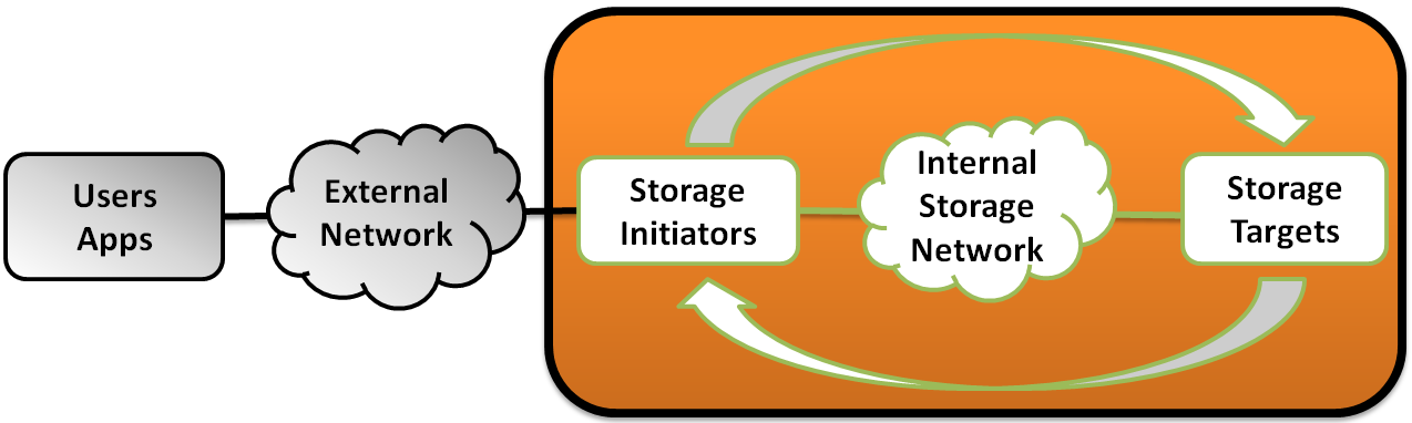The fact that the workload is steady means that whatever is transpiring over the black link connecting the orange blob with external world has fixed characteristics, throughput and latency wise. It is as if the lower parts (layers) of the apps – those that produce and consume I/Os – execute directly inside storage initiators without taking any resources. The I/Os get generated at application-defined rates and distributed across the cluster, with subsequent interactions over Internal Storage Network.

Now, if you stare at the picture for a few minutes you’ll start noticing then that the orange blob looks like an isolated system.

Well, it is in fact an isolated system in equilibrium.

“Isolated system” and “equilibrium” – this spells Physics. Could Physics help find answers to the Persistent Question?

On the one hand, distributed storage is not Physics – at least not in any practical sense, or maybe not just yet. On the other, the famous second law of thermodynamics has been successfully applied across boundaries, to, for instance, economic theory.

Which is why, even though the equilibrium of the picture above is not necessarily thermal – the idea kind of starts taking shape..

4. When the logarithm is a straight line

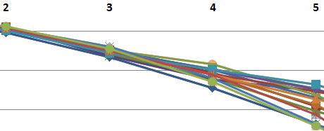
Time to cut to the chase. The idea is that large clusters tend to align themselves in state configurations oddly reminiscent of statistical mechanics. Here’s a plotted benchmark that corresponds to the commit 2a740a3 and shows logarithms of the probabilities for a clustered node to have a certain number of pending I/O requests – a certain queue depth.

The setup in this case includes 180 targets running reservations-based storage protocol that I’d previously called “Choosy Initiator”.

During the benchmark each storage target tracks durations of each specific queue depth (in nanoseconds). That is, for depths (0, 1, 2, 3, … max) each server counts the respective cumulative numbers of 1ns ticks. The resulting counters are then summed up over successive 1ms intervals, and the results converted to average cluster-wide probabilities:

where max is the maximum queue depth, and n(i) – total number of nanoseconds the targets had queue depth = i.

Hence, the chart below shows log(p(i)) for the observed range 0 – 8: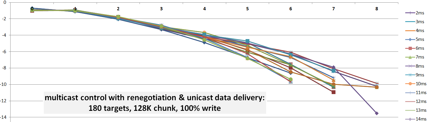Let p(i) be the probability for a target having exactly i reservations in its queue. The chart tells us that log(p(i)) trends close enough to a linear function:

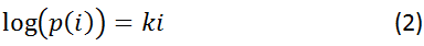
where k = -1.34 as per:

Wait, step back for a second. The linear dependency between log(p) and the reservation states could well be: a) not a line, b) a coincidence, c) a freaky coincidence, d) all of the above…

To be continued in part II.