What is the difference between storage cluster and multi-armed bandit (MAB)? This is not a trick question – to help answer it, think about this one: what’s common between MAB and Cloud configurations for big data analytics?
Henceforth, I’ll refer to these use cases as cluster, MAB, and Cloud configurations, respectively. The answer’s down below.
In storage clusters, there are storage initiators and storage targets that continuously engage in routine interactions called I/O processing. In this “game of storage” an initiator is typically the one that makes multi-choice load-balancing decisions (e.g., which of the 3 available copies do I read?), with the clear objective to optimize its own performance. Which can be pictured as, often rather choppy, diagram where the Y axis reflects a commonly measured and timed property: I/O latency, I/O throughput, IOPS, utilization (CPU, memory, network, disk), read and write (wait, active) queue sizes, etc.

Fig. 1. Choosy Initiator: 1MB chunk latencies (us) in the cluster of 90 targets and 90 initiators.
A couple observations, and I’ll get to the point. The diagram above is (an example of) a real-time time-series, where the next measured value depends on both the previous history and the current action. In the world of distributed storages the action consists in choosing a given target at a given time for a given (type, size) I/O transaction. In the world of multi-armed bandits, acting means selecting an arm, and so on. All of this may sound quite obvious, on one hand, and disconnected, on another. But only at the first glance.
In all cases the observed response carries a noise, simply because the underlying system is a bunch of physical machines executing complex logic where a degree of nondeterminism results, in part, from myriad micro-changes on all levels of the respective processing stacks including hardware. No man ever steps in the same river twice (Heraclitus).
Secondly, there always exists a true (latent, objective, black-box) function Y = f(history, action) that can potentially be inferred given a good model, enough time, and a bit of luck. Knowing this function would translate as the ability to optimize across the board: I/O performance – for storage cluster, gambling returns – for multi-armed bandits, $/IOPS ratio – for big data clouds. Either way, this would be a good thing, and one compelling reason to look deeper.
Thirdly and finally, a brute-force search for the best possible solution is either too expensive (for MAB, and Cloud configurations), or severely limited in time (which is to say – too expensive) for the cluster. In other words, the solution must converge fast – or be unfeasible.
The Noise
A wide range of dynamic systems operate in an environment, respond to actions by an agent, and generate serialized or timed output:

Fig. 2. Agent ⇔ Environment diagram.
This output is a function f(history, action) of the previous system states – the history – and the current action. If we could discover, approximate, or at least regress to this function, we could then, presumably, optimize – via a judicious choice of an optimal action at each next iteration…
And so, my first idea was: neural networks! Because, when you’ve got for yourself a new power, you better use it. Go ahead and dump all the cluster-generated time-series into neural networks of various shapes, sizes, and hyperparameters. Sit back and see if any precious latent f() shows up on the other end.
Which is exactly what I did, and well – it didn’t.
There are obstacles that are somewhat special and specific to distributed storage. But there’s also a common random noise that slows down the learning process, undermining its converge-ability and obfuscating the underlying system properties. Which is why the very second idea: get rid of the noise, and see if it helps!
To filter the noise out, we typically compute some sort of a moving average and say that this one is a real signal. Well, not so fast…
First off, averaging across time-series is a lossy transformation. The information that gets lost includes, for instance, the dispersion of the original series (which may be worse than Poissonian or, on the contrary, better than Binomial). In the world of storage clusters the index of dispersion may roughly correspond to “burstiness” or “spikiness” – an important characteristic that cannot (should not) be simplified out.
Secondly, there’s the technical question of whether we compute the average on an entire stream or just on a sliding window, and also – what would be the window size, and what about other hyperparameters that include moving weights, etc.
Putting all this together, here’s a very basic noise-filtering logic: Fig. 3. Noise filtering pseudocode.
This code, in effect, is saying that as long as the time-series fits inside the 3-sigma wide envelope around its moving average, we consider it devoid of noise and therefore we keep it as is. But, if the next data point ventures outside this “envelope”, we do a weighted average (line 3.b.i), giving it a slightly more credence and weight (0.6 vs 0.4). Which will then, at line 3.e, contribute to changing the first and the second moments based either on the entire timed history or on its more recent and separately configurable “window” (as in Fig. 1, which averages over a window of 10).
As a side: it is the code like this (and its numerous variations – all based on pure common sense and intuition) – that makes one wonder: why? Why are there so many new knobs (aka hyperparameters) per line of code? And how do we go about finding optimal values for those hyperparameters?..
Be as it may, some of the questions that emerge from Fig. 3 include: do we actually remove the noise? what is the underlying assumption behind the 3 (or whatever is configured) number of sigmas and other tunables? how do we know that an essential information is not getting lost in addition to, or maybe even instead of, “de-jittering” the stream?
All things being Bayesian
It is always beneficial to see a big picture, even at the risk of totally blowing the locally-observable one out of proportion ©. The proverbial big picture may look as follows:

Fig. 4. Bayesian inference.
Going from top to bottom, left to right:
- A noise filtering snippet (Fig. 3) implicitly relies on an underlying assumption that the noise is normally distributed – that it is Gaussian (white) noise. This is likely okay to assume in the cluster and Cloud configurations above, primarily due to size/complexity of the underlying systems and the working force of the Central Limit Theorem (CLT).
- On the other hand, the conventional way to filter out the noise is called the Kalman Filter, which, in fact, does not make any assumptions in re Gaussian noise (which is a plus).
- The Kalman filter, in turn, is based on Bayesian inference, and ultimately, on the Bayes’ rule for conditional probabilities.
- Bayesian inference (Fig. 4) is at the core of very-many things, including Bayesian linear regression (that scales!) and iterative learning in Bayesian networks (not shown); together with Gaussian (or normal) distribution Bayesian inference forms a founding generalization for both hidden Markov models (not shown) and Kalman filters.
- On the third hand, Bayesian inference happens to be a sub-discipline of statistical inference (not shown) which includes several non-Bayesian paradigms with their own respective taxonomies of methods and applications (not shown in Fig. 4).
- Back to the Gaussian distribution (top right in Fig. 4): what if not only the (CLT-infused) noise but the function f(history, action) itself can be assumed to be probabilistic? What if we could model this function as having a deterministic mean(Y) = m(history, action), with the Y=f() values at each data point normally distributed around each of its m() means?
- In other words, what if the Y = f(history, action) is (sampled from) a Gaussian Process (GP) – the generalization of the Gaussian distribution to a distribution over functions:

Fig. 5. Gaussian Process.
- There’s a fast-growing body of research (including already cited MAB and Cloud configurations) that answers Yes to this most critical question.
- But there is more…
- Since the sum of independent Gaussian processes is a (joint) GP as well, and
- since a Gaussian distribution is itself a special case of a GP (with a constant K=σ2I covariance, where I is the identity matrix), and finally,
- since white noise is an independent Gaussian
– the noise filtering/smoothing issue (previous section) sort of “disappears” altogether – instead, we simply go through well-documented steps to find the joint GP, and the f() as part of the above.
- When a Gaussian process is used in Bayesian inference, the combination yields a prior probability distribution over functions, an iterative step to compute the (better-fitting) posterior, and ultimately – a distinct machine learning technique called Bayesian optimization (BO) – the method widely (if not exclusively) used today to optimize machine learning hyperparameters.
- One of the coolest things about Bayesian optimization is a so-called acquisition function – the method of computing the next most promising sampling point in the process that is referred to as exploration-versus-exploitation.
- The types of acquisition functions include (in publication order): probability of improvement (PI), expected improvement (EI), upper confidence bound (UCB), minimum regret search (MRS), and more. In each case, the acquisition function computes the next optimal (confidence-level wise) sampling point – in the process that is often referred to as exploration-versus-exploitation.
- The use of acquisition functions is an integral part of a broader topic called optimal design of experiments (not shown). The optimal design tracks at least 100 years back, to Kirstine Smith and her 1918 dissertation, and as such does not explain the modern Bayesian renaissance.
- In the machine learning setting, though, the technique comes to the rescue each and every time the number of training examples is severely limited, while the need (or the temptation) to produce at least some interpretable results is very strong.
- In that sense, a minor criticism of the Cloud configurations study is that, generally, the performance of real systems under-load is spiky, bursty and heavily-tailed. And it is, therefore, problematic to assume anything-Gaussian about the associated (true) cost function, especially when this assumption is then tested on a small sample out of the entire “population” of possible {configuration, benchmark} permutations.
- Still, must be better than random. How much better? Or rather, how much better versus other possible Bayesian/GP (i.e., having other possible kernel/covariance functions), Bayesian/non-GP, and non-Bayesian machine learning techniques?
- That is the question.
Only a few remaining obstacles
When the objective is to optimize or (same) approximate the next data point in a time-series, both Bayesian and RNN optimizers perform the following 3 (three) generic meta-steps:
- Given the current state h(t-1) of the model, propose the next query point x(t)
- Process the response y(t)
- Update the internal state h(t+1)
Everything else about these two techniques – is different. The speed, the scale, the amount of engineering. The applicability, after all. Bayesian optimization (BO) has proven to work extremely well for a (constantly growing) number of applications – the list includes the already cited MAB and Cloud configurations, hyperparameter optimization, and more.
However. GP-based BO does not scale: its computational complexity grows as O(n3), where n is the number of sampled data points. This is clearly an impediment – for many apps. As far as storage clustering, the other obstacles include:
- a certain adversarial aspect in the relationships between the clustered “players”;
- a lack of covariance-induced similarity between the data points that – temporally, at least – appear to be very close to each other;
- the need to rerun BO from scratch every time there is a change in the environment (Fig. 2) – examples including changes in the workload, nodes dropping out and coming in, configuration and software updates and upgrades;
- the microsecond latencies that separate load balancing decisions/actions, leaving little time for machine learning.
Fortunately, there’s a bleeding-edge research that strives to combine the power of neural networks with the Bayesian power to squeeze the “envelope of uncertainty” around the true function (Fig. 6) – in just a few iterations:

Fig. 6. Courtesy of: Taking the Human Out of the Loop: A Review of Bayesian Optimization.
To be continued…

 Time t1 – everything is cool, t2 – a spike, a storm, a flood, a “Houston, we have a problem”, t3 – back to cool again.
 Or worse.
 Especially taking into account that TCP flows are mutually-independent, scheduling-wise.
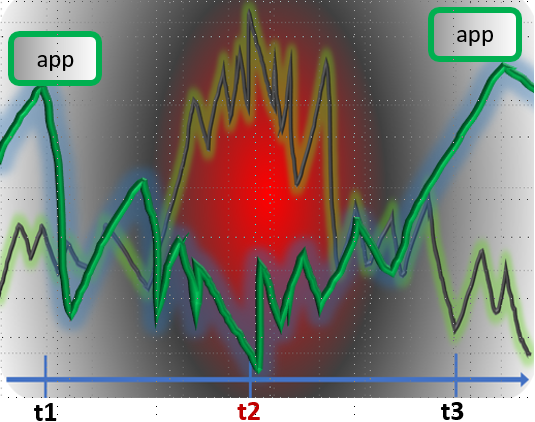 When it probably would – prior to t2 – send and receive some data. And then, more data at around and after t3. Which is fine, as long as the app in question could function without this data altogether and maybe (preferably) take advantage of having any of it, if available.
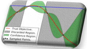


