The Proxy’s conundrum
In the end, group proxy must deliver: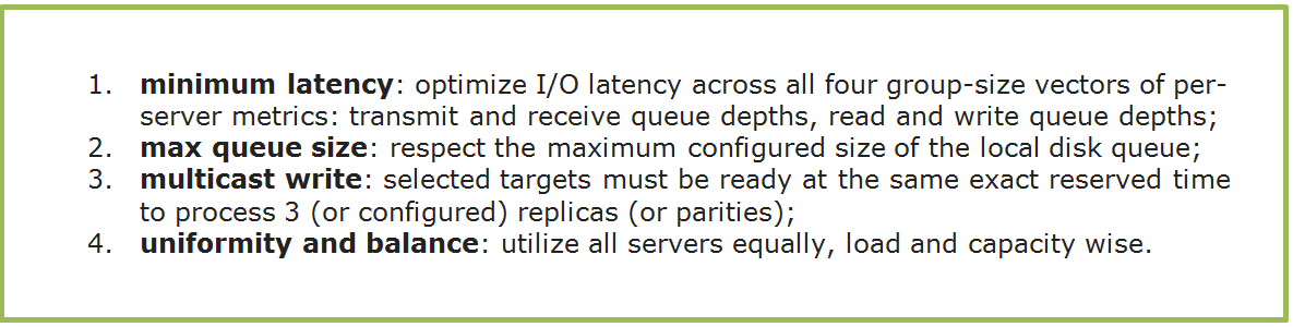 Requirements #2 and #3 are limiting, while #1 and (compound) #4 are optimizing, which also means that the proxy’s problem belongs to the vast field of multi-criteria decision making – aka vector optimization. This is a loosely named branch of computing where the domain-specific decision maker (DM) must be continuously taking multiple dynamic factors into account.
Most of the time the DM’s decisions will not maximize all factors/objectives simultaneously (see for instance Pareto optimality), which is especially true when the number of state variables is very large and the resulting behavior, even though deterministic at each of its state transitions, appears to be rather stochastic if not probabilistic.
Speaking of load balancing groups of servers, at any point in time the state of the group is described by a fixed number of variables that record and reflect the combination of network and disk resources already committed and scheduled by previous I/O requests. The following is generally true for all distributed storages where nodes have their own local (and locally owned) resources: each new I/O is effectively a “bump” in the utilization of the corresponding storage and network resource. Resource freeing process, on the other hand, is continuous and constant-speed – the resource-specific bandwidth or throughput.
The beauty of modeling, however, lies in the eye of beholder and in the immediacy of the results. Here’s a piece of model-generated log where the target/proxy T#46 makes a load-balancing selection for a newly arrived (highlighted) chunk: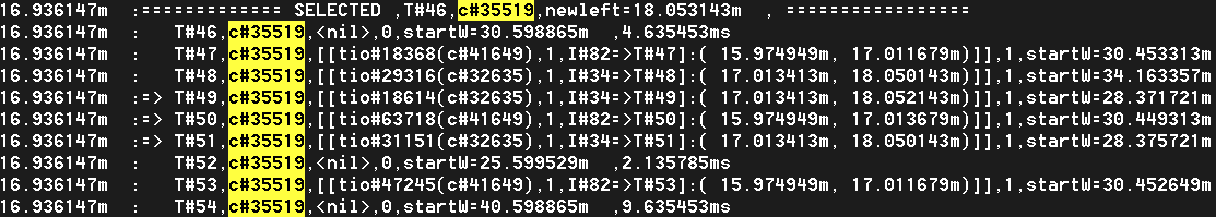 This log tells a story. At the 16.9..ms timestamp all targets in this group have pending requests referencing previously submitted/requested chunks. The model selects 3 targets denoted by ‘=>’ on the left, giving preference to the T#50. From the log we see that target T#52 was not selected even though it could ostensibly start writing (‘startW=’) the new chunk a bit earlier.
Runtime considerations of this sort where optimal write latency is weighed against other factors in play – is what I call the Proxy’s conundrum. Tradeoffs include the need to optimize and balance the reads, on one hand, while maintaining uniform distribution and balanced utilization, on another.
Group Tetris
OK, so each new I/O is effectively a “bump”. Figure 6 helps to visualize it with a group of six (horizontal axis), and the corresponding per-server pending data chunks (vertical axis). One unit on a vertical scale is the time to deliver one fixed-size chunk from initiator to target, or vise versa. Figure 6. Write request targeting a group of 6 storage servers
Proxy’s choice in this case indicates targets 1, 3, and 6, with a horizontal dashed line at the point in the timeline when the very first bit of the new chunk can cross respective local network interfaces.
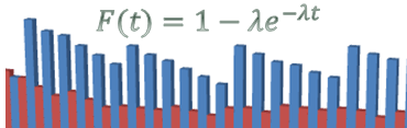
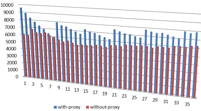
Now for a more complex (and realistic) visualization, here is a plotted benchmark where the proxied model is subjected to random 128K size, 50/50 read/write workload, and where frontend/backend of the cluster consists of 90 storage initiators and 90 targets, respectively. Each vertical step in the stacked bar chart captures newly received bytes and is exactly 100μs interval, with colored bars indicating the same exact moment in running time. Figure 7. Cumulative received bytes (vertical axis) measured in 100μs increments
One immediate observation: even though during a measured interval a given server receives almost nothing or nothing at all, overall as time progresses the 9 group members in this case find themselves more or less on the same cumulative (received-bytes) level. It appears that the model manages to avoid falling into the Pareto “trap”, whereby servers that did get utilized keep getting utilized even further.
It takes a handful of runs such as the one above, to start seeing a pattern. This pattern just happens to be reminiscent of a game of Tetris, where writes are blue, reads are green, and future is wide-open and uncharted:
About the Tail
In part I of this series I talked about fat-tailed latency distributions: why do we often see them in the distributed post-Dynamo world, and how to make them go away.
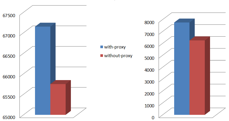
The chart: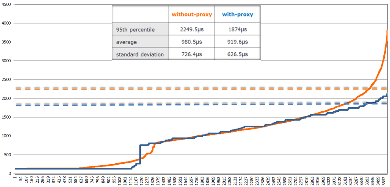 Figure 9. Write latencies (in microseconds)
shows proxied (blue) and proxy-less (orange) sorted write latencies under the same 128K, 50/50 workload, as well as 95th percentiles as horizontal dotted lines of respective coloring.
Not to jump to conclusions, but a (tentative) observation that can be drawn from this limited experiment (and a few others that I don’t show) is that load balancing a group of clustered servers makes things overall better. At the very least it makes the proverbial tail lighter and more subdued (so to speak). Not clear what’ll happen if the model runs through couple million chunks instead of 3,500 (above). But all in due time.
Optimizing the Future
Ultimately, the crux of the difference between proxy-less distributed system and its proxied counterpart is – information: load balancing proxy has just more of it as far as its group of servers is concerned, more than any given storage initiator at any time.
What’s next and where do we go from here? The following is a generalized 2-step sequence the proxy can run to optimize for the stated multi-objectives:
- identify R+K targets capable to execute new request with the best latency, where R is the required redundancy, K>0 is configurable, and R+K <= size of the load balancing group;
- apply the uniformity and balance criteria to each R-element subset of the R+K set.
Most intriguing aspect for me would be to see if the past I/Os can be used to optimize future ones. Or rather, not ‘if’ and not ‘how’ but ‘whether’ – whether it’d make a better than single-digit percentage difference in the performance.
Hence, the idea. The setup is a very large distributed cluster under a given stable workload. To compute the next step, load-balancing proxy utilizes a few previous I/Os, where a few is greater equal 2 and less equal, say, 16.
The proxy uses past I/Os to generate same number of future I/Os while preserving respective sizes, read/write ratios and relative arrival frequencies. Next, the proxy executes what is normally called a dry run.
Once all of the above is set and done, the proxy then selects those R targets out of (R+K) that provide for the optimal extrapolated future.
This of course assumes that the immediate past – the past defined in terms of I/O sizes, read/write ratios and relative arrival frequencies – has a good instructional value as far as the future. It usually does.
Post Scriptum
A zillion burning questions will have to remain out of scope. How will the proxied model perform for unicast datapath? What’s the performance delta between the with and without-proxy protocols which otherwise must be totally apples-to-apples comparable? What are the upper and lower bounds of this delta, and how would it depend on average chunk/block sizes, read/write ratios, sizes of the load balancing group, ratios between the network and disk bandwidths?..
One thing is clear to me, though. Thinking that initiator-driven hashed distribution means uniform and balanced distribution – this thinking is wrong (it is also naïve, irresponsible and borderlines on tastelessness, but that’s just me going off the record). This text tries to make a step. Stuff can be modeled, certain ideas tested – quickly..