Lifecycle management

There’s a set of topics in system management that can often be found under alternative subtitles:
“graceful termination and cleanup”, “shutting down and restarting”, “adding/removing members”, “joining and leaving cluster”, and similar.

Any discussion along those lines typically involves state transitions, so let’s go ahead and name the states (and transitions).

To put things in perspective, this picture is about a node (not shown) in an aistore cluster (not shown). Tracking it from the top downwards, first notice a state called “maintenance mode”. “Maintenance mode” constitutes maybe the most gentle, if you will, way of removing a node from the operating cluster.

When in maintenance, the node stops keep-alive heartbeats but remains in the cluster map and remains connected. That is, unless you disconnect or shut it down manually (which would be perfectly fine and expected).

Next is “shutdown”. Graceful shutdown can also be achieved in a single shot, as indicated by one of those curly arrows in the picture’s left: “online” => “shutdown”.

When in “shutdown”, a node can easily get back and rejoin the cluster at any later time. It’ll take two steps, not one – see the blue arrows on the picture’s right where RESTART must be understood as a deployment-specific operation (e.g., kubectl run).

Both “maintenance” and “shutdown” involve a certain intra-cluster operation called “global rebalance” (aka “rebalance”).

But before we talk about it in any greater detail, let’s finish with the node’s lifecycle. The third and final special state is “decommission”. Loosely synonymous with cleanup (a very thorough cleanup, as it were), “decommission” entails:

  • migrating all user data the node is storing to other nodes that are currently “online” – the step that’s followed by:
  • partial or complete cleanup of the node in question, whereby the complete cleanup further entails:
  • removing all AIS metadata, all configuration files, and – last but not least – user data in its entirety.

Needless to say, there’s no way back out of “decommission” – the proverbial point of no return. To rejoin the cluster, a decommissioned node will have to be redeployed from scratch, but then it would be a totally different node, of course…

Cluster

There’s one question that absolutely cannot wait: how to “terminate” or “cleanup” a cluster? Here’s how:

$ ais cluster decommission --rm-user-data --yes

The above command will destroy an existing cluster – completely and utterly, no questions asked. It can be conveniently used in testing/benchmarking situations or in any sort of non-production environment – see --help for details. It also executes very fast – Ctrl-C’s unlikely to help in case of change-of-mind…

Privileges

Full Disclosure: all lifecycle management commands and all associated APIs require administrative privileges. There are, essentially, three ways:

  • deploy the cluster with authentication disabled:
$ ais config cluster auth --json
    "auth": {
        "secret": "xxxxxxxx",
        "enabled": false
    }
  • use integrated AuthN server that provides OAuth 2.0 compliant JWT and a set of easy commands to manage users and roles (with certain permissions to access certain clusters, etc.);
  • outsource authorization to a separate, centralized (usually, LDAP-integrated) management system to manage existing users, groups, and mappings.

Rebalance

Conceptually, aistore rebalance is similar to what’s often called “RAID rebuild”. The underlying mechanics would be very different but the general idea is the same: user data massively migrating from some nodes in a cluster (or disks in an array) to some other nodes (disks), and vice versa.

In aistore, all the migration (aka “rebalancing”) that’s taking in place is the system response to a lifecycle event that’s already happened or is about to happen. In fact, it is the response to satisfy a singular purpose and a single location-governing rule that simply states: user data must be properly located.

Proper location

For any object in a cluster, its proper location is defined by the current cluster map and locally – on each target node – by the locally configured target’s mountpaths.

In that sense, the “maintenance” state, for instance, has its beginning – when the cluster starts rebalancing, and the post-rebalancing end, whereby the corresponding sub-state get recorded in a new version of the cluster map, which then gets safely distributed across all nodes, etc., etc.

Next section gives an example and further clarifies the notion of maintenance sub-states.

Quick example

Given a 3-node single-gateway cluster, we go ahead and shut down one of the nodes:

$ ais cluster add-remove-nodes shutdown <TAB-TAB>
p[MWIp8080]   t[ikht8083]   t[noXt8082]   t[VmQt8081]

$ ais cluster add-remove-nodes shutdown t[ikht8083] -y

Started rebalance "g47" (to monitor, run 'ais show rebalance').
t[ikht8083] is shutting down, please wait for cluster rebalancing to finish

Note: the node t[ikht8083] is _not_ decommissioned - 
it remains in the cluster map and can be manually
restarted at any later time (and subsequently activated via 'stop-maintenance' operation).

Once the command is executed, notice the following:

$ ais show cluster
...
t[ikht8083][x]   -   -   -   -   maintenance

At first, maintenance will show up in red indicating a simple fact that data is expeditiously migrating from the node (which is about to leave the cluster).

A visual cue, which is supposed to imply something like: “please don’t disconnect, do not power off”.

But eventually, if you run the command periodically:

$ ais show cluster --refresh 3

or a few times manually – eventually show cluster will report that rebalance (“g47” in the example) has finished and the node t[ikht8083] – gracefully terminated. Simultaneously, maintenance in the show output will become non-red.

The takeaway: global rebalance runs its full way before the node in question is permitted to leave. If interrupted for any reason whatsoever (power-cycle, network disconnect, new node joining, cluster shutdown, etc.) – rebalance will resume and will keep going until the governing condition is fully and globally satisfied.

Summary

lifecycle operationCLIbrief description
maintenance modestart-maintenanceThe most lightweight way to remove a node. Stop keep-alive heartbeats, do not insist on metadata updates – ignore the failures. For advanced usage options, see --help.
shutdownshutdownSame as above, plus node shutdown (aisnode exit).
decommissiondecommissionSame as above, plus partial (metadata only) or complete (both data and AIS metadata) cleanup. A decommissioned node is forever “forgotten” – removed from the cluster map.
remove node from cluster mapais advanced remove-from-smapStrictly intended for testing purposes and special use-at-your-own-risk scenarios. Immediately remove the node from the cluster and distribute updated cluster map with no rebalancing.
take node out of maintenancestop-maintenanceUpdate the node with the current cluster-level metadata, re-enable keep-alive, run global rebalance. Finally, when all succeeds, distribute updated cluster map (where the node shows up “online”).
join new node (ie., grow cluster)joinEssentially, same as above: update the node, run global rebalance, etc.

Assorted notes

Normally, a starting-up AIS node (aisnode) will use its local configuration to communicate with any other node in the cluster and perform what’s called self-join. The latter does not require a join command or any other explicit administration.

Still, the join command can be useful when, for instance, node is misconfigured or started as a standby.

When rebalancing, the cluster remains fully operational and can be used to read and write data, list, create, and destroy buckets, run jobs, and more. In other words, none of the listed lifecycle operations requires downtime. The persistent idea is that users never notice…

References

Finding the right storage system

What are the odds that you find the right storage system to run all the workloads that need to be running and to forever sustain all the apps that consume storage? Given the current state of the art, what would be your chances of doing so today?

Apart from being existential, the question also appears to be formalizable. Meaning that it can be approached with a certain degree of scientific rigor and scrupulousness. Of course, I’m talking about the Drake equation.

The Drake equation is a probabilistic argument used to estimate the number of active, communicative extraterrestrial civilizations in the Milky Way galaxy. Since its 1961 publication, and notwithstanding constructive criticism (see, for instance,The Drake Equation Is Broken; Here’s How To Fix It“) the equation proved to be usable across wide range of application domains.

Perhaps the most popular application of Drake is estimating one’s chances to find true love (variations: girlfriend, boyfriend, soulmate, BFF).

Given a massive body of work on the subject I’ll have to limit citations to maybe just one: the 2008 paper “Why I don’t have a girlfriend” where Peter Backus clearly and succinctly explains a) how to apply Drake, and b) why at the time of the writing he didn’t have a girlfriend.

Back to storage systems though – equipped with Drake’s methodology, the question of finding the one and only storage system can be factorized (step 1), with the probabilities of each factor estimated (step 2), and fed into the equation (step 3) to generate an estimate. Consider a real-life example, whereby the storage system in question features:

  1. SDS: software stack on commodity x86 servers
  2. Price $0.10/GB or below that covers hardware + software + 5 years of support
  3. Petascale clustering with 1PB usable today and growing to 100PB later in 2019
  4. Storage media: hard drives
  5. Linearity: must scale close to linear with each added node and each added spindle
  6. HA: must be highly available
  7. Tiering: unlimited
  8. Data redundancy: both local (RAID1/5/6/10) and replicated
  9. AI: built-in accelerations for AI workloads

A quick look at the above reveals the truth: the chance of locating a match is probably low.

Indeed, at the time of this writing, the Wikipedia’s computer storage category includes a total of about 150 companies. Even if we super-generously give each of the 9 factors an average 0.5 probability, the resulting (150 * 1/512) can only be interpreted as: oops, doesn’t exist.

There are numerous ways to confirm the first suspicion. For instance, given the limited dataset of 150, we could run Monte Carlo simulations by randomly selecting storage companies and filling-in samples, e.g.:

Storage company X.Y.Z. SDS: No Petascale: No Price: Not cheap Commodity x86: No HA: Yes

Having accumulated enough samples to generate confidence intervals, we then compute the odds, find them depressingly low, and resort to finding some peace in the pure logic of this exercise, a consolation similar to the one Peter Backus found years ago.

We could also take a more conventional route which (conventionally) entails: reviewing datasheets, meeting with vendors, gathering references, reading Top-N IDC and Gartner reports, and then again reviewing the product datasheets. Here, for instance, are the top 13 companies from the IDC Worldwide Object Storage 2018 – we could take this report and painstakingly fill-in a 13-by-9 comparison table with those companies in the rows and the distinguishing characteristics in the columns (I will leave this as an exercise for the reader).

IDC-WOS-2018

Source: The Register

Most likely, though, if nothing even remotely plausible comes up on the first day or two of screening, referencing, and filling out comparison tables, the chance (of finding the right storage system) must be considered extremely slim. The storage system that you need, seek, and depend upon may not exist.

Or, stated differently, the storage system that you really need may really not exist.

It’ll be hard to come to terms with this statement – the process will usually take anywhere between three to nine months. Eventually, though, the dilemma will crystallize as a simple binary choice: to build or not to build?

This is a tough choice to make. Here’s one possible answer. Why does it work for the 9 (nine) factors listed above and where does it go from there – that will be another story and a different time.

Neural Networks for Storage Games

Even though machine learning is used extensively and successfully in numerous distinct areas, the idea to apply it to hardcore (fast) datapaths may seem farfetched. Which is also why I’m currently looking at the distributed storage use case where storage nodes employ different I/O load balancing strategies. Some of these nodes run neural networks, others – maybe a more conventional logic. Some of these strategies perform better than others, but only when they compete against their deterministic counterparts. The text below is only scratching the surface, of course:

Neural Networks for Storage Games (pdf)

Bayesian Optimization for Clusters

What is the difference between storage cluster and multi-armed bandit (MAB)? This is not a trick question – to help answer it, think about this one: what’s common between MAB and Cloud configurations for big data analytics?

Henceforth, I’ll refer to these use cases as cluster, MAB, and Cloud configurations, respectively. The answer’s down below.

In storage clusters, there are storage initiators and storage targets that continuously engage in routine interactions called I/O processing. In this “game of storage” an initiator is typically the one that makes multi-choice load-balancing decisions (e.g., which of the 3 available copies do I read?), with the clear objective to optimize its own performance. Which can be pictured as, often rather choppy, diagram where the Y axis reflects a commonly measured and timed property: I/O latency, I/O throughput, IOPS, utilization (CPU, memory, network, disk), read and write (wait, active) queue sizes, etc.


Fig. 1. Choosy Initiator: 1MB chunk latencies (us) in the cluster of 90 targets and 90 initiators.

A couple observations, and I’ll get to the point. The diagram above is (an example of) a real-time time-series, where the next measured value depends on both the previous history and the current action. In the world of distributed storages the action consists in choosing a given target at a given time for a given (type, size) I/O transaction. In the world of multi-armed bandits, acting means selecting an arm, and so on. All of this may sound quite obvious, on one hand, and disconnected, on another. But only at the first glance.

In all cases the observed response carries a noise, simply because the underlying system is a bunch of physical machines executing complex logic where a degree of nondeterminism results, in part, from myriad micro-changes on all levels of the respective processing stacks including hardware. No man ever steps in the same river twice (Heraclitus).

Secondly, there always exists a true (latent, objective, black-box) function Y = f(history, action) that can potentially be inferred given a good model, enough time, and a bit of luck. Knowing this function would translate as the ability to optimize across the board: I/O performance – for storage cluster, gambling returns – for multi-armed bandits, $/IOPS ratio – for big data clouds. Either way, this would be a good thing, and one compelling reason to look deeper.

Thirdly and finally, a brute-force search for the best possible solution is either too expensive (for MAB, and Cloud configurations), or severely limited in time (which is to say – too expensive) for the cluster. In other words, the solution must converge fast – or be unfeasible.

The Noise

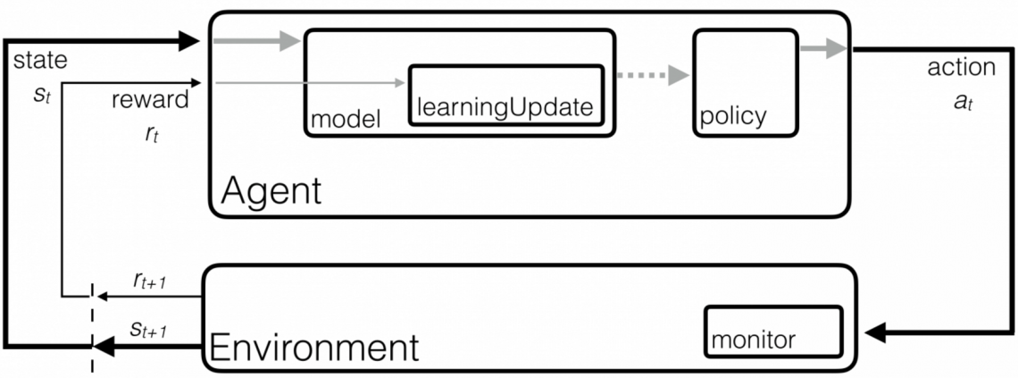
A wide range of dynamic systems operate in an environment, respond to actions by an agent, and generate serialized or timed output:

Fig. 2. Agent ⇔ Environment diagram.
This output is a function f(history, action) of the previous system states – the history – and the current action. If we could discover, approximate, or at least regress to this function, we could then, presumably, optimize – via a judicious choice of an optimal action at each next iteration…

And so, my first idea was: neural networks! Because, when you’ve got for yourself a new power, you better use it. Go ahead and dump all the cluster-generated time-series into neural networks of various shapes, sizes, and hyperparameters. Sit back and see if any precious latent f() shows up on the other end.

Which is exactly what I did, and well – it didn’t.

There are obstacles that are somewhat special and specific to distributed storage. But there’s also a common random noise that slows down the learning process, undermining its converge-ability and obfuscating the underlying system properties. Which is why the very second idea: get rid of the noise, and see if it helps!

To filter the noise out, we typically compute some sort of a moving average and say that this one is a real signal. Well, not so fast…

First off, averaging across time-series is a lossy transformation. The information that gets lost includes, for instance, the dispersion of the original series (which may be worse than Poissonian or, on the contrary, better than Binomial). In the world of storage clusters the index of dispersion may roughly correspond to “burstiness” or “spikiness” – an important characteristic that cannot (should not) be simplified out.

Secondly, there’s the technical question of whether we compute the average on an entire stream or just on a sliding window, and also – what would be the window size, and what about other hyperparameters that include moving weights, etc.

Putting all this together, here’s a very basic noise-filtering logic:Fig. 3. Noise filtering pseudocode.

This code, in effect, is saying that as long as the time-series fits inside the 3-sigma wide envelope around its moving average, we consider it devoid of noise and therefore we keep it as is. But, if the next data point ventures outside this “envelope”, we do a weighted average (line 3.b.i), giving it a slightly more credence and weight (0.6 vs 0.4). Which will then, at line 3.e, contribute to changing the first and the second moments based either on the entire timed history or on its more recent and separately configurable “window” (as in Fig. 1, which averages over a window of 10).

As a side: it is the code like this (and its numerous variations – all based on pure common sense and intuition) – that makes one wonder: why? Why are there so many new knobs (aka hyperparameters) per line of code? And how do we go about finding optimal values for those hyperparameters?..

Be as it may, some of the questions that emerge from Fig. 3 include: do we actually remove the noise? what is the underlying assumption behind the 3 (or whatever is configured) number of sigmas and other tunables? how do we know that an essential information is not getting lost in addition to, or maybe even instead of, “de-jittering” the stream?

All things being Bayesian

It is always beneficial to see a big picture, even at the risk of totally blowing the locally-observable one out of proportion ©. The proverbial big picture may look as follows:

Fig. 4. Bayesian inference.
Going from top to bottom, left to right:

  1. A noise filtering snippet (Fig. 3) implicitly relies on an underlying assumption that the noise is normally distributed – that it is Gaussian (white) noise. This is likely okay to assume in the cluster and Cloud configurations above, primarily due to size/complexity of the underlying systems and the working force of the Central Limit Theorem (CLT).
  2. On the other hand, the conventional way to filter out the noise is called the Kalman Filter, which, in fact, does not make any assumptions in re Gaussian noise (which is a plus).
  3. The Kalman filter, in turn, is based on Bayesian inference, and ultimately, on the Bayes’ rule for conditional probabilities.
  4. Bayesian inference (Fig. 4) is at the core of very-many things, including Bayesian linear regression (that scales!) and iterative learning in Bayesian networks (not shown); together with Gaussian (or normal) distribution Bayesian inference forms a founding generalization for both hidden Markov models (not shown) and Kalman filters.
  5. On the third hand, Bayesian inference happens to be a sub-discipline of statistical inference (not shown) which includes several non-Bayesian paradigms with their own respective taxonomies of methods and applications (not shown in Fig. 4).
  6. Back to the Gaussian distribution (top right in Fig. 4): what if not only the (CLT-infused) noise but the function f(history, action) itself can be assumed to be probabilistic? What if we could model this function as having a deterministic mean(Y) = m(history, action), with the Y=f() values at each data point normally distributed around each of its m() means?
  7. In other words, what if the Y = f(history, action) is (sampled from) a Gaussian Process (GP) – the generalization of the Gaussian distribution to a distribution over functions:


Fig. 5. Gaussian Process.

  1. There’s a fast-growing body of research (including already cited MAB and Cloud configurations) that answers Yes to this most critical question.
  2. But there is more…
  3. Since the sum of independent Gaussian processes is a (joint) GP as well, and
    • since a Gaussian distribution is itself a special case of a GP (with a constant K=σ2I covariance, where I is the identity matrix), and finally,
      • since white noise is an independent Gaussian

– the noise filtering/smoothing issue (previous section) sort of “disappears” altogether – instead, we simply go through well-documented steps to find the joint GP, and the f() as part of the above.

  1. When a Gaussian process is used in Bayesian inference, the combination yields a prior probability distribution over functions, an iterative step to compute the (better-fitting) posterior, and ultimately – a distinct machine learning technique called Bayesian optimization (BO) – the method widely (if not exclusively) used today to optimize machine learning hyperparameters.
  2. One of the coolest things about Bayesian optimization is a so-called acquisition function – the method of computing the next most promising sampling point in the process that is referred to as exploration-versus-exploitation.
  3. The types of acquisition functions include (in publication order): probability of improvement (PI), expected improvement (EI), upper confidence bound (UCB), minimum regret search (MRS), and more. In each case, the acquisition function computes the next optimal (confidence-level wise) sampling point – in the process that is often referred to as exploration-versus-exploitation.
  4. The use of acquisition functions is an integral part of a broader topic called optimal design of experiments (not shown). The optimal design tracks at least 100 years back, to Kirstine Smith and her 1918 dissertation, and as such does not explain the modern Bayesian renaissance.
  5. In the machine learning setting, though, the technique comes to the rescue each and every time the number of training examples is severely limited, while the need (or the temptation) to produce at least some interpretable results is very strong.
  6. In that sense, a minor criticism of the Cloud configurations study is that, generally, the performance of real systems under-load is spiky, bursty and heavily-tailed. And it is, therefore, problematic to assume anything-Gaussian about the associated (true) cost function, especially when this assumption is then tested on a small sample out of the entire “population” of possible {configuration, benchmark} permutations.
  7. Still, must be better than random. How much better? Or rather, how much better versus other possible Bayesian/GP (i.e., having other possible kernel/covariance functions), Bayesian/non-GP, and non-Bayesian machine learning techniques?
  8. That is the question.

Only a few remaining obstacles

When the objective is to optimize or (same) approximate the next data point in a time-series, both Bayesian and RNN optimizers perform the following 3 (three) generic meta-steps:

  • Given the current state h(t-1) of the model, propose the next query point x(t)
  • Process the response y(t)
  • Update the internal state h(t+1)

Everything else about these two techniques – is different. The speed, the scale, the amount of engineering. The applicability, after all. Bayesian optimization (BO) has proven to work extremely well for a (constantly growing) number of applications – the list includes the already cited MAB and Cloud configurations, hyperparameter optimization, and more.

However. GP-based BO does not scale: its computational complexity grows as O(n3), where n is the number of sampled data points. This is clearly an impediment – for many apps. As far as storage clustering, the other obstacles include:

  • a certain adversarial aspect in the relationships between the clustered “players”;
  • a lack of covariance-induced similarity between the data points that – temporally, at least – appear to be very close to each other;
  • the need to rerun BO from scratch every time there is a change in the environment (Fig. 2) – examples including changes in the workload, nodes dropping out and coming in, configuration and software updates and upgrades;
  • the microsecond latencies that separate load balancing decisions/actions, leaving little time for machine learning.

Fortunately, there’s a bleeding-edge research that strives to combine the power of neural networks with the Bayesian power to squeeze the “envelope of uncertainty” around the true function (Fig. 6) – in just a few iterations:

Fig. 6. Courtesy of: Taking the Human Out of the Loop: A Review of Bayesian Optimization.

To be continued…

Storage Cluster in Thermal Equilibrium (part II)

In essence, Part I of this post stipulates that distribution of states in large clusters can be approximated without making any assumptions on what kind of distribution it is in the first place.

The claim, hypothetical at this point, is that storage clusters under certain conditions must be conforming to the laws of statistical mechanics (StMch). The narrow version of the same claim relates strictly to the mathematics used in StMch.

Since the remaining part II came out pretty lengthy, heavy on math, and densely populated with equations, I’m including it here as a separate PDF.

TL;DR.

The results, I’d say, are inconclusive-but-promising. Part of being “inconclusive” is simply – not enough data, too early to say. Testing the theory on larger, 10K nodes and beyond, clusters seems like a no-brainer. However. Out of all possible whats-next ideas and steps my first preference would be to check out this theory not directly on the clustered nodes but instead on the load-balancing groups and their group-wide aggregated states..

Docker Detour

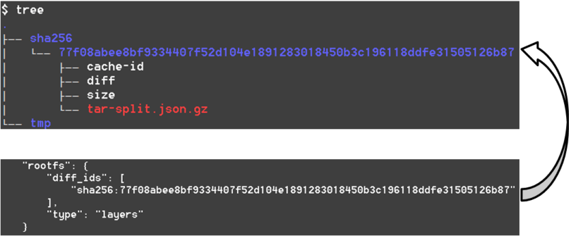
Docker keeps fascinating me, purely as a use case. From the image hosting perspective, there are a couple things that are missing in its current stage of development. The biggest and the most obvious one is – a shared,  distributed, and deduplicated store for both image manifests (image metadata) and layer content (the data).

Due to the immutable sha256-protected nature of both the related complexity is about 3 orders of magnitude lower than (this complexity would look like for) anything less specialized.

Distributing the content-hashed and stacked stuff like this:

docker-det-1

Read More »

Storage Cluster in Thermal Equilibrium (part I)

Mathematics is the art of giving the same name to different things.

Henri Poincare

1. Life’s most persistent question

The question is: how to compute distribution of states of clustered nodes in a large distributed cluster running a steady workload? The cluster is fully distributed, and:boltz-txt1None of this is uncommon. For one thing, we live at a time of ever-exploding problem sizes. Bigger problems lead to bigger clusters with nodes that, when failed, get replaced wholesale.

And small stuff. For instance, eventually consistent storage is fairly common knowledge today.  It is spreading fast, with clumps of apps (including venerable big data and NoSQL apps) growing and stacking on top.

Those software stacks enjoy minimal centralized processing (and often none at all), which causes CAP-imposed scalability limits to get crushed. This further leads to even bigger clusters, where nodes run complex stateful software, etcetera.

Why complex and stateful, by the way? The most generic sentiment is that the software must constantly evolve, and as it evolves its complexity and stateful-ness increases. Version (n+1) is always more complex and more stateful than the (n) – and if there are any exceptions that I’m not aware of, they only confirm the rule. Which fully applies to storage, especially due to the fact that this particular software must keep up with the avalanche of hardware changes. There’s a revolution going on. The SSD revolution is still in full swing and raging, with SCM revolution right around the corner. The result is millions of lines of code, and counting. It’s a mess.

Read More »

The Better Protocol (part II)

The Proxy’s conundrum

In the end, group proxy must deliver:gproxy-textboxRequirements #2 and #3 are limiting, while #1 and (compound) #4 are optimizing, which also means that the proxy’s problem belongs to the vast field of multi-criteria decision making – aka vector optimization. This is a loosely named branch of computing where the domain-specific decision maker (DM) must be continuously taking multiple dynamic factors into account.

Most of the time the DM’s decisions will not maximize all factors/objectives simultaneously (see for instance Pareto optimality), which is especially true when the number of state variables is very large and the resulting behavior, even though deterministic at each of its state transitions, appears to be rather stochastic if not probabilistic.

Speaking of load balancing groups of servers, at any point in time the state of the group is described by a fixed number of variables that record and reflect the combination of network and disk resources already committed and scheduled by previous I/O requests. The following is generally true for all distributed storages where nodes have their own local (and locally owned) resources: each new I/O is effectively a “bump” in the utilization of the corresponding storage and network resource. Resource freeing process, on the other hand, is continuous and constant-speed – the resource-specific bandwidth or throughput.

The beauty of modeling, however, lies in the eye of beholder and in the immediacy of the results. Here’s a piece of model-generated log where the target/proxy T#46 makes a load-balancing selection for a newly arrived (highlighted) chunk:gproxy-log2This log tells a story. At the 16.9..ms timestamp all targets in this group have pending requests referencing previously submitted/requested chunks. The model selects 3 targets denoted by ‘=>’ on the left, giving preference to the T#50. From the log we see that target T#52 was not selected even though it could ostensibly start writing (‘startW=’) the new chunk a bit earlier.

Runtime considerations of this sort where optimal write latency is weighed against other factors in play – is what I call the Proxy’s conundrum. Tradeoffs include the need to optimize and balance the reads, on one hand, while maintaining uniform distribution and balanced utilization, on another.

Group Tetris

OK, so each new I/O is effectively a “bump”. Figure 6 helps to visualize it with a group of six (horizontal axis), and the corresponding per-server pending data chunks (vertical axis). One unit on a vertical scale is the time to deliver one fixed-size chunk from initiator to target, or vise versa.gproxy-groupsixFigure 6. Write request targeting a group of 6 storage servers

Proxy’s choice in this case indicates targets 1, 3, and 6, with a horizontal dashed line at the point in the timeline when the very first bit of the new chunk can cross respective local network interfaces.

Now for a more complex (and realistic) visualization, here is a plotted benchmark where the proxied model is subjected to random 128K size, 50/50 read/write workload, and where frontend/backend of the cluster consists of 90 storage initiators and 90 targets, respectively. Each vertical step in the stacked bar chart captures newly received bytes and is exactly 100μs interval, with colored bars indicating the same exact moment in running time.gproxy-rxbytesFigure 7. Cumulative received bytes (vertical axis) measured in 100μs increments

One immediate observation: even though during a measured interval a given server receives almost nothing or nothing at all, overall as time progresses the 9 group members in this case find themselves more or less on the same cumulative (received-bytes) level. It appears that the model manages to avoid falling into the Pareto “trap”, whereby servers that did get utilized keep getting utilized even further.

It takes a handful of runs such as the one above, to start seeing a pattern. This pattern just happens to be reminiscent of a game of Tetris, where writes are blue, reads are green, and future is wide-open and uncharted:gproxy-tetris

About the Tail

In part I of this series I talked about fat-tailed latency distributions: why do we often see them in the distributed post-Dynamo world, and how to make them go away.

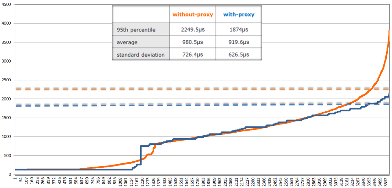
The chart:gproxy-latencytailFigure 9. Write latencies (in microseconds)

shows proxied (blue) and proxy-less (orange) sorted write latencies under the same 128K, 50/50 workload, as well as 95th percentiles as horizontal dotted lines of respective coloring.

Not to jump to conclusions, but a (tentative) observation that can be drawn from this limited experiment (and a few others that I don’t show) is that load balancing a group of clustered servers makes things overall better. At the very least it makes the proverbial tail lighter and more subdued (so to speak). Not clear what’ll happen if the model runs through couple million chunks instead of 3,500 (above). But all in due time.

Optimizing the Future

Ultimately, the crux of the difference between proxy-less distributed system and its proxied counterpart is – information: load balancing proxy has just more of it as far as its group of servers is concerned, more than any given storage initiator at any time.

What’s next and where do we go from here? The following is a generalized 2-step sequence the proxy can run to optimize for the stated multi-objectives:

  1. identify R+K targets capable to execute new request with the best latency, where R is the required redundancy, K>0 is configurable, and R+K <= size of the load balancing group;
  2. apply the uniformity and balance criteria to each R-element subset of the R+K set.

Most intriguing aspect for me would be to see if the past I/Os can be used to optimize future ones. Or rather, not ‘if’ and not ‘how’ but ‘whether’ – whether it’d make a better than single-digit percentage difference in the performance.

Hence, the idea. The setup is a very large distributed cluster under a given stable workload. To compute the next step, load-balancing proxy utilizes a few previous I/Os, where a few is greater equal 2 and less equal, say, 16.

The proxy uses past I/Os to generate same number of future I/Os while preserving respective sizes, read/write ratios and relative arrival frequencies. Next, the proxy executes what is normally called a dry run.

Once all of the above is set and done, the proxy then selects those R targets out of (R+K) that provide for the optimal extrapolated future.

This of course assumes that the immediate past – the past defined in terms of I/O sizes, read/write ratios and relative arrival frequencies – has a good instructional value as far as the future. It usually does.

Post Scriptum

A zillion burning questions will have to remain out of scope. How will the proxied model perform for unicast datapath? What’s the performance delta between the with and without-proxy protocols which otherwise must be totally apples-to-apples comparable? What are the upper and lower bounds of this delta, and how would it depend on average chunk/block sizes, read/write ratios, sizes of the load balancing group, ratios between the network and disk bandwidths?..

One thing is clear to me, though. Thinking that initiator-driven hashed distribution means uniform and balanced distribution – this thinking is wrong (it is also naïve, irresponsible and borderlines on tastelessness, but that’s just me going off the record). This text tries to make a step. Stuff can be modeled, certain ideas tested – quickly..

The Better Protocol (part I)

It’s been noted before that Ceph benchmarks produce results that are lower than expected. Take for instance the most recent FAST’16 [BTrDB] paper (quote):

<snip> Applying this backpressure early prevents Ceph from reaching pathological latencies. Consider Figure 9a where it is apparent that not only does the Ceph operation latency increase with the number of concurrent write operations, but it develops a long fat tail, with the standard deviation exceeding the mean. Furthermore, this latency buys nothing, as Figure 9b shows that the aggregate bandwidth plateaus…

fat-tailed2

The above is indeed a textbook case (courtesy of [BTrBD]) of fat-tailed distribution, the one that deviates from its mean with high probability having either undefined or unbounded standard deviation (sigma). But wait..  the fat-tailed latency problem is by no means Ceph-specific.

Disclaimer:

Nexenta produces a competing solution that is called NexentaEdge. Secondly, needless to say that opinions expressed in this text are strictly and solely my own.

There are multiple reasons to single-out Ceph, the most researched and likely the most widely used general-purpose distributed storage stack. Ceph is an open source project as well, open for in-depth reviews. CRUSH remains one of the best content distribution algorithms. In sum, Ceph is as close as it gets to being a representative of the current generation – generation of post-Dynamo distributed storage systems.

The problem though affects majority of fully-distributed storage systems. To add insult to injury, it cannot be easily bug-fixed. The fat-tailed, heavy-tailed, long-tailed latency problem is in fact the other side of the uniformly-distributed “coin”.

The Conflict

A distributed storage cluster consists of multiple user-facing Storage Initiators (henceforth, “initiators”) and multiple reading/writing Storage Targets (“targets”).

Both initiators and targets execute concurrently and in parallel, the former – app requests, the latter – disk I/Os. Often {initiator + target} pairs are bundled as dual-function daemons within their respective clustered nodes – case in point (hyper)converged architectures, but not only.

The defining characteristic of a fully distributed cluster is that the path from an initiator to a target is direct. The datapath does not “cross” any central authority.

There is a lot of varying intelligence typically built into existing initiators, to help them decide where and how to route I/O requests. This intelligence, however, executes in the management and control (error processing) planes leaving fast path data distribution decisions totally up to the clustered frontend – to a given storage initiator.

This is exactly why do we have the following generic conflict – in Ceph, and in Swift, and in others.

the-conflict

Figure 1. The Conflict

The figure depicts initiators A and B simultaneously reaching out to the same target Y. Since there’s no metadata server (MDS), centralized arbiter/load-balancer or any other kind of central logic in the datapath, each initiator simply goes ahead and reaches out based on the best information it had at the time.

From the target Y’s perspective, however, it just happened so that the two requests arrive in rapid succession within the same interval – the interval that, on average, corresponds to a single I/O request under a given workload (aka inter-arrival time).

Visualize a storage cluster consisting of identical nodes, where user data is uniformly distributed by multiple initiators, thus providing, on average, well-balanced resource utilization: CPU, network, I/O bandwidth and disk capacity of individual targets. Here’s the pertinent question: what is the probability of a conflict depicted above, where storage targets are forced to handle multiple requests within a single interval of time.

Poisson approximation

In statistics, a Poisson experiment must have the following defining properties:

  • The experiment results in outcomes that can be classified as successes or failures.
  • The average number of successes that occurs in a specified time interval is known.
  • The probability that a success will occur is proportional to the size of the interval.
  • The probability that a success will occur in an extremely small interval is virtually zero.

To make the connection, I’ll go out on a limb and say this: a very large fully distributed storage cluster under a fully random workload and sufficiently large working set can be (***) approximated as a massive Poisson experiment-generating machine. Whereby the target’s chances to see two or more I/O requests during a time interval t would compute as:poisson-aTherefore, at a sustained workload of, say, modest 10K per-target IOPS, the average inter-I/O interval would be 100μs. Given uniform distribution of I/O requests, the probability of two or more requests within this average 100μs interval is precisely:poisson-b1Meaning, for at least a quarter of all 100μs long intervals each target should expect to handle at least 2 interval-sharing requests. And in about 2% of all time the number spikes up to 4 or more, as per:poisson-2

Since storage clusters normally run many hours, days and months at a time, the 2% must be understood as accumulated minutes and hours of random 4x spikes.

Uniform distributions fair well when the cluster is – on average – underutilized. But if and when the load and pressure grows beyond 50% utilization and the resulting average per-I/O interval shrinks proportionally, then very quickly and quite frequently the targets are required to execute well above the average, and ultimately beyond their provisioned maximum bandwidth.

How frequently? At 50% utilization each clustered target must be expected to run at least 2 times faster than its own maximum performance at least 2% of the time. That is, assuming of course that the entire storage system can be modeled as a Poisson process.

But can it?

(***) Poisson processes are memoryless and, simultaneously, stateless – the two fine and abstract properties  that are definitely not present in any real-life storage situation, distributed or local. Things get cached and journaled, aggregated and deduplicated. Generally, storage nodes (like the ones shown on Fig. 1) at any point in time have a wealth of accumulated state to deal with.

There are also multiple ways by which the targets may share their feedback and their own state with initiators, and each of these “ways” would create an additional state in the corresponding cluster-representing Markov’s chain which ultimately can become rather huge and unwieldy..

My sense though is (and here I’m frankly on shaky grounds) that given the (a, b, c, d) assumptions below, the Poisson approximation is valid and does hold.

(a) large fully distributed storage cluster;
(b) random workload;
(c) massive working set that tramples any and every attempt to cache;
(d) direct and uniform initiator ⇒ target distribution of data.

At the very least it gives an idea.

Synthetic Idea

To recap:

  1. Distributed clustering whereby a certain segment of datapath and/or metadata path is centralized – is a legacy that does not scale;
  1. Total decentralization of both data and metadata I/O processing via uniform and direct initiator-to-target distribution is the characterizing property of modern-time storage architectures. It works great but only under low to medium utilizations.

The idea is to inject a bit of centralization into the otherwise fully and uniformly distributed cluster, to provide for scale and, simultaneously, true balance under stress. An example of one such protocol follows, along with benchmarks and comparison in the second (and separate) part of this text.

On the Go

The implementation involves homegrown SURGE framework that is written in Go. I’m using Go mostly due to its built-in goroutines and channels – the language primitives that were invented to quickly write pieces of communicating logic that independently and concurrently run inside distributed “nodes”. As many nodes as your heart desires..

In SURGE each storage node (initiator or target) is a separate lightweight thread: a goroutine. The framework connects all configured nodes bi-directionally, via a pair of per node (Tx, Rx) Go channels. At model’s startup all clustered nodes (of this model) get automatically connected and ready to Go: send, receive and handle events and I/O requests from all other nodes.

There are various infrastructure classes (aka types) and utilities reused by the previously implemented models, for instance a rate bucket type that helps implement network and disk bandwidth limitations, and many more (see for instance the entry on this site titled Choosy Initiator).

Each SURGE model is an event-distributing event-driven machine. Quoting one previous text on this site:

Everything that happens in a modeled world is a result of prior events, and the result of everything-that-happens is: new events. Event timings define the progression of Time itself..

Clustered configuration is practically unlimited. Each data frame and each control packet is a separate timed event over a separate peer-to-peer channel. The number of events exchanged during a single given benchmark is, frankly, mind-blowing – it blows my mind, it still does.

Load Balancing Groups with group leaders

The new model (main piece of the source code here) represents a storage cluster that consists of load balancing groups of storage targets. Group size is configurable, with the only guideline that it corresponds to the required redundancy – due to the fact that each group acts as a whole as far as storing/retrieving redundant content.

The protocol leverages multicast replication of user data, and control plane that is, at least in part, terminated by a per-group selected leader, aka Group Proxy (from here on simply: proxy). In the simulation a proxy is a storage target with a minimal ID inside its own group.

Let’s see how it works without going yet into much detail – picture below illustrates the write/put sequence:write-seq2

Figure 2. Write Sequence

  • initiator A sends write request to the target X, which is also (in its second role) – a group leader or a proxy responsible(*) for its group G;
  • target X then performs a certain non-trivial computation based on outstanding previous requests – from all initiators;
  • this results in two back-to-back transactions from/by the target X:
    1. write reservation sent to the initiator A, and
    2. auto-reservations sent to the selected targets in the group G, made on behalf of those selected targets (note that target X depicted here includes itself into the selection process);
  • given the reservation time window and the list of selected targets, initiator A then multicasts data –one data frame at a time, at provisioned link bandwidth (which is configurable, with control bandwidth and overhead factored-in);
  • once the entire payload is received, each of the selected targets updates proxy X with its current size of its disk queue;
  • finally, when the payload is safely stored, each selected target sends an ACK to the initiator A indicating: done.

As far as read/get, the pipeline starts with the read request delivered to all members of the group (Fig. 3). The idea is the same though: it is up to the proxy to decide who’s handling the read. More exactly:read-seq2

Figure 3. Read Sequence

  • initiator A maps or hashes the read (or rather name of the file, ID of the chunk, LBA of the block, etc.) onto a group G, and then sends the request to all members of this same G;
  • target X which happens to be the group leader (or, proxy) receives read responses from those targets in the group that store the corresponding data;
  • once target X collects all or some(*) responses, it makes an educated decision. Similar to the write case (Fig. 2), this decision involves looking at all previous-but-still-outstanding I/O requests, and computing the best target to perform the read;
  • finally, selected target sends the data back to the requesting initiator, which prior to this point would have been already updated with its (the target’s) ID and the time (deadline) to expect the read to commence.

Notice that in both read and write cases it is the group proxy that performs behind-the-scenes tracking of who-does-what-when for the entire group. The proxy, effectively, is listening on everything transpiring on the group-targeting control plane, and makes inline I/O routing decisions on behalf of the rest of group members.

Instead of conclusions

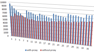
Wrapping up: one quick summary chart that shows the respective with group proxy and without group proxy benchmark-average performances expressed as chunks-per-second. The 50% read, 50% write workload is directed into 90 simulated targets by as many initiators, and the chunk sizes are 128K on the left, and 1M on the right, respectively:

summary-perf

Figure 4. Average throughput

And here’s the throughput over time, for the same 50%/50% workload and 1MB chunk size:

throughput-1M

Figure 5. Throughput for 1M chunk

This experiment corresponds to the 1ae1388 commit. In the second upcoming part of the series I’ll try to show how exactly the comparison is done, and why exactly the results are what they are.


Evolution, some say, moves is spiraling circles and cycles. Software paradigms evolve and mutate, with every other iteration reintroducing stuff that was buried deep in the past. Or so it seems.

Post-Dynamo clusters that have evolved in forms of distributed block arrays, object storage clusters and NoSQL databases, reject any centralized processing in the datapath. There is a multifaceted set of interesting limitations that comes with that. What could be the better protocol? To be continued…