Choosy Initiator

March 20, 2016March 20, 2016 Alex Aizman1 Comment

In a fully distributed storage cluster (FDSC), one possible design choice for a new storage protocol is resource reservation (RR). There are certain distinct challenges though, when working out an optimal RR schema. On the storage initiator side, one critical question that arises is whether to accept an RR response a.k.a. a bid from a given target for a given I/O request. Or, alternatively, try to renegotiate, in hopes of getting a better reservation.

The absolutely best reservation is, of course, the one that allows I/O in question to start immediately and execute at full throttle.

Hence, choosy initiator in the title, the storage initiator that grapples with the dilemma: go ahead and accept possibly suboptimal arrangement, or renegotiate. The latter inevitably comes with the risk to receive future reservations that are even more delayed.

To bet or not to bet, that is the question. To find out, I’ve used SURGE: a discrete open source event simulation framework written in Go (https://golang.org/doc/). The source includes a bunch of concrete protocol models (that run) and the usual README to get started.

OK, let’s do some definitions.

FDSC and RR

The three key aspects of a FDSC are self-containment, full connectivity, and hashed distribution:

Self-containment: each clustered node is a sole owner of its local resources: disks, CPU, memory, and link bandwidth;

Any-to-any: all nodes are interconnected through non-blocking, no-drop network core;

Hashed memoryless distribution: a given I/O request is mapped or hashed to a number of storage target. For writes, the number of targets must be equal or greater than the required redundancy. This I/O mapping/hashing operation does not depend on the history and on any of the previously executed I/O requests (hence, memoryless).

Note separately that the letter ‘S’ in FDSC also reads as “symmetric”. In symmetric clusters, each node performs a dual role of storage initiator and storage target simultaneously.

For now let’s just say that large fully distributed clusters counting hundreds or thousands initiators and targets require a different intra-cluster transport. That’s #1, the point that maybe does not sound very controversial. To add controversy (just for the heck of it), here’s the point #2: for large and super-large FDSC it makes a lot of sense to use RR based transport protocols. One of the key proof points boils down to convergence.

Convergence time is the time it takes for existing link-sharing (path-sharing) flows to converge on their respective optimal rates when a new flow is being added or an existing flow removed. All things being equal, each of the N flows eventually must take 1/Nth of the total bandwidth.

Figure 12 in the research paper at http://goo.gl/JUlijH shows DCTCP convergence times.

Red flow (below) is added after the blue flow has reached its steady and close-to-optimal state. The research estimates DCTCP convergence times on a 10GE network ranging anywhere from 229*d to 770*d, where d is the propagation delay. This is a considerable time corresponding to several fully transferred 128K payloads even for a very favorable (as far as speedy convergence) value of d in the order of few microseconds.

choosy-fig1 — Figure 1. DCTCP convergence (courtesy DCTCP research)

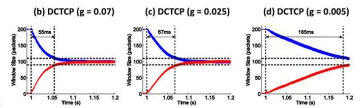
In presence of multiple flows the picture gets substantially more messy but the bigger point is: irrespective of the particular link-sharing transport, during the time N flows are converging from (N-1) or (N+1), they all execute at sub-optimal rates resulting in overall sub-optimal network utilization. Hence, an appeal of the RR approach: eliminate resource sharing. Utilization time slots are simply negotiated. There will be no unexpected start-IO, complete-IO, and add-flow, delete-flow events in the middle.

If there exists anything similar in real life, that could be a timeshare ownership. On the networking side examples include RSVP in its unicast and multicast realizations (RFC2205).

In all cases (including timeshare) and independently of the concrete resource reservation protocol, each successful RR negotiation comes with a time window in combination with a full set of requested targets resources – for exclusive usage (during a given time window) by a given pending request (emphasis on exclusive). For each I/O request, there is a natural progression:

I/O request =>
   potential targets =>
      RR negotiation(s) =>
          data flows to/from ...

This results in network flows executing as prescribed by non-overlapping time windows granted in turn by the respective selected targets.

To bet or not to bet

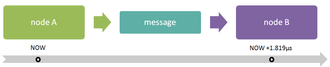
The figure below shows one possible “resource reservation, renegotiated” (RRR) scenario:

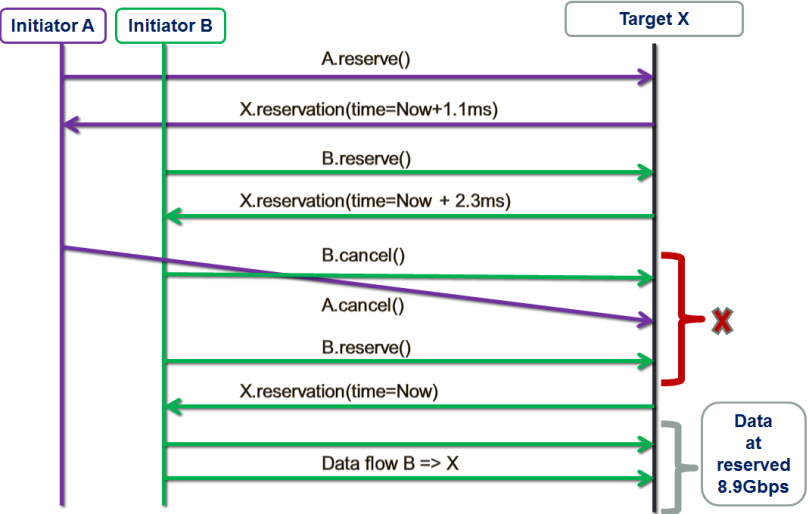
There are two storage initiators: purple A and green B. The initiators are trying to establish data flows with the same target X at approximately the same time.

First, initiator A tentatively reserves target X for a window starting 1.1ms later (from now), which roughly corresponds to the time target X needs to complete a (presumably) already queued 1MB transaction (not shown here).

Next, initiator B tentatively reserves X for the adjacent X’s time window at 2.3ms from now. Red X on the picture indicates the decision point.

In this example, instead of accepting whatever is presented to it at the moment, B decides that 2.3ms is too much of a delay and cancels. Simultaneously, A cancels as well, possibly because it has obtained more attractive bids from other storage targets that are not shown here. This further results in B getting the optimal reservation and utilizing it right away.

Simulation

The idea that at least sometimes it does make sense to take a risk and renegotiate requires proof. Fortunately, with SURGE we can run massive simulations to find out.

Replicast is a one FDSC-friendly RR-based protocol that was previously described – see for instance SNIA presentation Beyond Consistent Hashing and TCP.

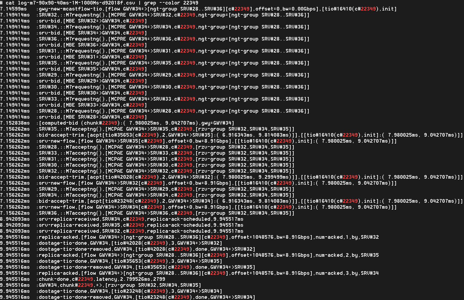
Replicast-H (where H stands for hybrid) entails multicast control plane and unicast data. Recall that RR negotiation is a part of the reservations-based protocol control plane. When running a hybrid version of the Replicast, we negotiate up to (typically) 3 successive time windows to perform a write. We then often see the following picture:

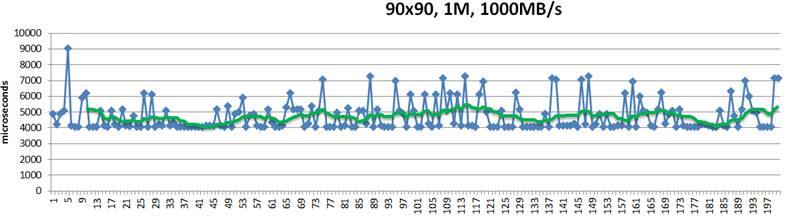
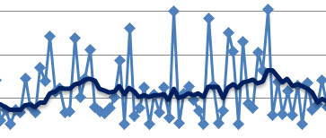
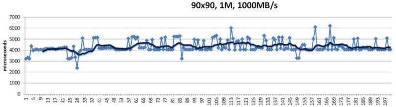
choosy-fig3 — Figure 3. Reservations without renegotiation

This above is a 200-point random sample that details latencies of 1MB size chunks written into their hashed target destinations. Green trendline in the middle shows 10-point moving average. This is a “plain” Replicast-H benchmark where each target’s bid is taken at a face value and never renegotiated.

The cluster in this case combines 90 targets and 90 storage initiators with targets operating at 1000MB/s disk throughput. Finally, there is a non-blocking no-drop 10Gbps that connects each target with each initiator.

In the simulation above 10% of the bandwidth is statically allocated for control traffic. With 1% accounting for network headers and miscellaneous overhead, that leaves 8.9Gbps for (pure) data.

In the idealistic conditions when a given initiator does not have any competition from others, the times to execute a 1MB write to a single target would be, precisely:

Network: 941.482µs
Disk: 1ms

Given 3 copies, the request could (ideally) be fully executed in slightly more than 4 milliseconds, including control handshakes and acknowledgements.

There is, however, inevitably a competition resulting in reservation conflicts and delays, and further manifesting itself in occasional end-to-end spikes up to 7ms latency and beyond – see the picture above.

In depth analysis of traces (that I will skip here) indicates that, indeed, one possible reason for the spikes is that initiators accept reservations too early. For instance, the initiator that executed the #5 in the sample (Fig. 3) could likely do better.

Unicast delivery with renegotiation

This “with renegotiation” flavor of the protocol adds a new configuration variable that currently defaults to 3 times RTT on the control plane:

Note: to go directly to the github source, click this and other similar code fragments. At runtime, this model will double the wait time and renegotiate reservations if and when the actual waiting time (denoted as ‘idletime’ below) exceeds the current value:

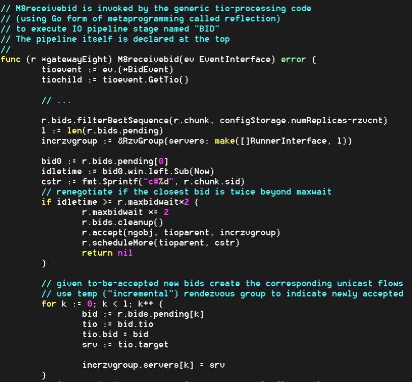
In addition, since 3 times RTT is just a crude initial guess, each modeled gateway (a.k.a. storage initiator) recomputes its value (‘r.maxbidwait’ in the code) for the next write request, averaging the previous value and the current one:

What happens after the first few transactions is that each initiator independently computes an objective average delay and from there on renegotiates only when the newly collected reservations collectively result in substantially bigger delay (in other words, the initiator renegotiates only when it “thinks” it could get a better deal).

Here’s the SURGE-simulated result for apples-to-apples identical configuration that runs 90 storage initiators and 90 storage targets, etc.:

choosy-fig4 — Figure 4. Reservations with renegotiation

Notice that there are no 7ms spikes anymore. They are simply gone.

Conclusions, briefly

For differently sized chunks and disk/backend throughputs, the average improvement ranges from 8% to 20%:

choosy-fig5 — Figure 5. 128K chunks, 400MB/s disk (left) and 1000MB/s disk (right)

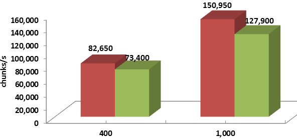
Legend-wise, red columns depict the “with renegotiation” version.

choosy-fig6 — Figure 6. 1MB chunks, 400MB/s disk (left) and 1000MB/s disk (right)

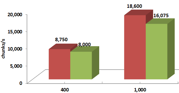
Thus, taking a risk does seem to pay off: RR based protocol where storage initiators are “choosy” and at least sometimes renegotiate their reservations outperforms its prior version.

SURGE: performance modeling for distributed systems

February 11, 2016 Alex Aizman

Foreword

As far as distributed system and storage software, finding out how it'll perform at scale - is hard.

Expensive and time-consuming as well, often impossible. When there are the first bits to run, then there’s maybe one, two hypervisors at best (more likely one though). That’s a start.

Early stages have their own exhilarating freshness. Survival is what matters then, what matters always. Questions in re hypothetical performance at 10x scales sound far-fetched, almost superficial. Answers are readily produced – in flashy powerpoints. The risk however remains, carved deep into the growing codebase, deeper inside the birthmarks of the original conception. Risk that the stuff we’ll spend next two, three years to stabilize will not perform.

The Goal

The goal is modeling the performance of a distributed system of any size (emphasis on modeling, performance and any size). Which means – uncovering the behavioral patterns (periodic spike-downs and, generally, any types of pseudo-regular irregularities), charting throughputs and latencies and their respective distributions concealed behind performance averages. And tails of those distributions, those that are in the single-digit percentile ranges.

Average throughput, average IOPS, average utilization, average-anything is not enough – we need to see what is really going on. For any scale, any configuration, any ratios of: clients and clustered nodes, network bandwidth and disk throughput, chunk/block sizes, you name it.

Enter SURGE, discrete event simulation framework written in Go and posted on GitHub. SURGE translates (admittedly, with a certain effort) as Simulator for Unsolicited and Reservation Group based and Edge-driven distributed systems. Take it or leave it (I just like the name).

Go aka golang, on the other hand, is a programming language¹ ².

Go

Go is an open source programming language introduced in 2007 by Rob Pike et al. (Google). It is a compiled, statically typed language in the tradition of C with garbage collection, runtime reflection and CSP-style concurrent programming.

CSP stands for Communicating Sequential Processes, a formal language, or more exactly, a notation that allows to formally specify interactions between concurrent processes. CSP has a history of impacting designs of programming languages.

Runtime reflection is the capability to examine and modify the program’s own structure and behavior at runtime.

Go’s reflection appears to be very handy when it comes to supporting IO pipeline abstractions, for example. But more about that later. As far as concurrency, Rob Pike’s presentation is brief and to the point imho. To demonstrate the powers (and get the taste), let’s look at a couple lines of code:

play.golang.org/p/B7U_ua0bzk

In this case, notation 'go function-name' causes the named function to run in a separate goroutine – a lightweight thread and, simultaneously, a built-in language primitive.

Go runtime scheduler multiplexes potentially hundreds of thousands of goroutines onto underlying OS threads.

The example above creates a bidirectional channel called messages (think of it as a typed Unix pipe) and spawns two concurrent goroutines: send() and recv(). The latter run, possibly on different processor cores, and use the channel messages to communicate. The sender sends random ASCII codes on the channel, the receiver prints them upon reception. When 10 seconds are up, the main goroutine (the one that runs main()) closes the channel and exits, thus closing the child goroutines as well.

Although minimal and simplified, this example tries to indicate that one can maybe use Go to build an event-distributing, event-driven system with an arbitrary number of any-to-any interconnected and concurrently communicating players (aka actors). The system where each autonomous player would be running its own compartmentalized piece of event handling logic.

Hold on to this visual. In the next section: the meaning of Time.

Time

In SURGE every node of a modeled cluster runs in a separate goroutine. When things run in parallel there is generally a need to go extra length to synchronize and sequence them. In physical world the sequencing, at least in part, is done for us by the laws of physics. Node A sending message to remote node B can rest assured that it will not see the response from node B prior to this sent message being actually delivered, received, processed, response created, and in turn delivered to A.

The corresponding interval of time depends on the network bandwidth, rate of the A ⇔ B flow at the time, size of the aforementioned message, and a few other utterly material factors.

That’s in the physical world. Simulated clusters and distributed models cannot rely on natural sequencing of events. With no sequencing there is no progression of time. With no progression there is no Time at all – unless…

Unless we model it. For starters let’s recall an age-old wisdom: time is not continuous (as well as, reportedly, space). Time rather is a sequence of discrete NOWs: one indivisible tick (of time) at a time. Per quantum physics the smallest time unit could be the Planck time ≈5.39*10^-44s although nobody knows for sure. In modeling, however, one can reasonably ascertain that there is a total uneventful void, literally nothing between NOW and NOW + 1.

In SURGE, the smallest indivisible tick of time is 1 nanosecond, a configurable default.

In a running operating physical cluster each NOW instant is filled with events: messages ready to be sent, messages ready to be received, events being handled right NOW. There are also en route messages and events sitting in disk and network queues and waiting for their respective future NOWs.

Let’s for instance imagine that node A is precisely NOW ready to transmit a 8KB packet to node B:

Given full 10Gbps of unimpeded bandwidth between A and B and the trip time, say, 1µs, we can then with a high level of accuracy predict that B will receive this packet (819ns + 1µs) later, that is at NOW+1.819µs as per the following:

play.golang.org/p/RZpYY_hNnQ

In this snippet of modifiable-and-runnable code, the local variable sizebits holds the number of bits to send or receive while bwbitss is a link bandwidth, in bits per second.

Time as Categorical Imperative

Here’s a statement of correctness that, on the face of it, may sound trivial. At any point in time all past events executed in a given model are either already fully handled and done or are being processed right now.

A past event is of course an event scheduled to trigger (to happen) in the past: at (NOW-1) or earlier. This statement above in a round-about way defines the ticking living time:

At any instant of time all past events did already trigger.

And the collateral:

Simulated distributed system transitions from (NOW-1) to NOW if and only when absolutely all past events in the system did happen.

Notice that so far this is all about the past – the modeled before. The after is easier to grasp:

For each instant of time all future events in the model are not yet handled - they are effectively invisible as far as designated future handlers.

In other words, everything that happens in a modeled world is a result of prior events, and the result of everything-that-happens is: new events. Event timings define the progression of Time itself. The Time in turn is a categorical imperative – a binding constraint (as per the true statements above) on all events in the model at all times, and therefore on all event-producing, event-handling active players – the players that execute their own code autonomously and in parallel.

Timed Event

To recap. Distributed cluster is a bunch of interconnected nodes (it always is). Each node is an active Go player in the sense that it runs its own typed logic in its own personal goroutine. Nodes continuously generate events, assign them their respective computed times-to-trigger and fan them out onto respective Go channels. Nodes also continuously handle events when the time is right.

By way of a sneak peek preview of timed events and event-driven times, here’s a life of a chunk (a block of object’s data or metadata) in one of the SURGE’s models:

The time above runs on the left, event names are abbreviated and capitalized (e.g. MCPRE). With hundreds and thousands of very chatty nodes in the model, logs like this one become really crowded really fast.

In SURGE framework each and every event is timed, and each timed event implements the following abstract interface:

type EventInterface interface {
    GetSource() RunnerInterface
    GetCreationTime() time.Time
    GetTriggerTime() time.Time
    GetTarget() RunnerInterface
    GetTio() *Tio
    GetGroup() GroupInterface
    GetSize() int
    IsMcast() bool
    GetTioStage() string
    String() string
}

This reads as follows. There is always an event source, event creation time and event trigger time. Some events have a single remote target, others are targeting a group (of targets). Event’s source and event’s target(s) are in turn clustered nodes themselves that implement (RunnerInterface).

All events are delivered to their respective targets at prescribed time, as per the GetTriggerTime() event’s accessor. The Time-defining imperative (above) is enforced with each and every tick of time.

In the next installment of SURGE series: ping-pong model, rate bucket abstraction, IO pipeline and more.

Embracing and Abandoning ZFS

December 18, 2015 Caitlin Bestler

If you are not familiar with ZFS, you should be. It is the best local file system ever developed.

It’s also likely to retain that title forever, because improving the local file system is not where the storage industry’s head is at these days. Distributed storage is the only way to scale-out to the degree that storage now requires.

My first design for Object Storage at Nexenta sought to leverage ZFS as one implementation of a “Local File System” superclass. It could bring benefits to both our Object Storage clusgter and to OpenStack Swift. This was a natural progression with evolutionary design. Nexenta is a ZFS company and we were very familiar with ZFS. We wanted to take advantage of the protection provided by ZFS within one server with distributed data protection. We dubbed this the “2+2” strategy. I presented the idea at the OpenStack Folsom summit.

The key advantage that ZFS enabled was the aibity to mix local replication with network replication, as summarized by the following two slides from that presentation:

OpenStackCCOW5

The obstacles to this approach proved to be too high. Relying on two network replicas where each machine keeps a high reliability mirror (“2 by 2”) can only achieve the same availability if you have two network ports on each storage server. Without dual network ports the loss of a single network interface leaves you only a single failure from losing access to data.

But dual ports are a concept that virtualization management simply does not want to understand. It wants a single Ethernet link to a single storage node. They either work as a complete unit, or they do not. A “2×2” solution requires tracking nodes that are in “limping” states such as knowing when a storage node is only reachable by one of its two links. Keeping track of the state of each server as being either “working”, “limping” or “dead” sound simple enough, but just “working” or “dead” is a lot simpler. There are other conditions that can put a storage device in a “limping” state where it can be read but should not be written to, such as a drive that is starting to fail. But this is the only thing that would require the management plane to add this concept.

Management plane developers hate adding more concepts when 90% of the world is happy without the additional work. So that wasn’t going anywhere.

We also realized that multicast UDP was a much better solution. Rather than battling to get network management improved so that we could go from 2 excess deliveries to 1 excess delivery we could just use multicast UDP and end up with 0 excess deliveries.

All of these issues were actually minor compared to the challenges of providing high performance object storage using Python.

Basically, it does not work.

Swift advocates will claim otherwise, but they are trying to con you that Object Storage should not be expected to be as high performance as SAN or NAS storage. I don’t buy that line of thinking.

There were several new ideas that we wanted to incorporate in the design, all of which will be covered in later blogs.

Totally decentralized control and namespaces.
Using multicast communications rather than point-to-point protocols such as TCP/IP.
Avoiding the constraints of Consistent Hashing.
Truly embracing Key/Value storage, top-to-bottom.

But there were also a lot that we wanted to inherit from ZFS – building upon ideas sometimes works better than directly reusing the code via modularized or layered architectures. Those eternal ZFS ideas, or at least some of them, are:

Copy-on-Write: never overwrite in-use data

```
Never Trust Storage Devices
```
```
Always be Consistent on Disk
```

Use Transaction Logs to Improve Performance

```
Use Snapshots and Clones
```
```
Replication Is Important
```
```
"Rampant Layering Violation"
```

Copy-on-Write

ZFS never overwrites in-use data. It writes new data, and then references the new data. The new object storage system would end up taking this even farther. Each new chunk has its content written exactly once. It can be replicated as needed, but a chunk once written is never updated.

Never Trust Storage Devices

It is not enough to respond to errors when disks report them. You need to validate the data read versus checksums stored elsewhere.

The new object storage system uses cryptographic hashes of each chunk’s payload to identify, locate and validate each chunk.

Always Be Consistent on Disk

The easiest way to always be consistent on what is written to persistent storage is to never write any data which a later action can invalidate.

The CCOW (Cloud Copy-on-Write) object storage system does not rely on any information stored about any chunk other than its cryptographic hash identifier.

Use Transaction Logs to Improve Performance

ZFS relies upon transaction logs to maintain its “always consistent on disk” goal. The data on disk is consistent, after you apply the pending transactions in the log after a sudden reboot. Updating the root after every transaction is the only other way to always be consistent on disk, and that would require far too many disk writes.

NexentaEdge uses the same technique to allow eventual update of related data structures after a new Version Manifest is written. It cuts the number of disk writes required before an acknowledgement of a Version Manifest Put transaction nearly in half.

Use Snapshots and Clones

ZFS creates snapshots by not deleting them. It can turn them into clones by simply allowing new version forks to branch from there.

Keeping this with a distributed object system was a challenge, but we came up with a method of truly snapshotting a distributed set of metadata. To push the photo analogy it is a true snapshot that captures the system state at one instant, it just needs to be developed before you can see the picture. I’ll describe that in a later blog.

Replication Is Important

How a system replicates data after it is put is not an afterthought. ZFS features snapshot driven replication. That feature is retained by NexentaEdge, just using NexentaEdge snapshots instead.

“Rampant Layering Violation”

Perhaps the most important lesson is an inherited attitude.

ZFS was accused of being a “Rampant Layering Violation”. Jeff Bonwick’s response (https://blogs.oracle.com/bonwick/entry/rampant_layering_violation) was that it was merely more intelligent layering that picked more effective divisions of responsibilities.

NexentaEdge will likely be accused of far worse layering violations.

The Replicast protocol considers storage distribution and network utilization at the same time.
Since the end user ultimately pays for both we see nothing wrong with optimizing both of them.
This is still layered – we only optimize traffic on the storage network. It is physically or logically (VLAN) separated from other networking. Optimizing the storage network for storage is just common sense.

Embracing by Abandoning

NexentaEdge storage servers use key value storage, whether physical or a software simulation of key/value storage. This is the simplest API for copy-on-write storage to use. While it might have been possible to define a key/value ZVol it just isn’t worth the effort. There is too little left of single machine ZFS left to make it worth building NexentaEdge on top of ZFS.

The ideas of ZFS, however, inspired the entire design effort.

BIER vs Transactional Subset Multicasting – An interesting case of differing perspectives.

October 28, 2015December 3, 2015 Caitlin Bestler

BIER

As noted in my previous blog on Transactional Subset Multicasting a distributed object cluster greatly benefits from push-mode multicasting. The sender determines the set of recipients rather than the recipients joining a group. Having the listeners join the multicast group adds a round-trip delay to every join. For a distributed storage cluster a dynamic group would have to be formed for each chunk put. That would typically be every 128 KB to 2 MB. That would be expensive even if IGMP/MLD joins executed promptly. They do not.

The only thing that is slower than IGMP/MLD joins are IGMP/MLD leaves. There is only minimal harm in not instantly shutting off an end stations reception of a stream it has lost interest in. But when you are trying to manage exactly which packets are delivered via which edge links you need the Leaves to process just as quickly as the Joins.

So naturally I was very interested in BIER. The NexentaEdge application more needs a short list of destinations, but a bitmap can be fairly efficient. BIER can even narrow the mapping to a “sub-domain” or a subset of a sub-domain’s bitmap using a “Subset Identifier” (SI). The bottom line is that each Negotiating Group could be mapped to a 64-bit bitmap. A single 64-bit map is shorter than a list of IPV6 addresses, so header space would not have been a problem.

Not That Straight Forward

While BIER looked like an interesting alternate solution to push multicasting I kept getting confused reading the BIER drafts. They seemed amazingly tolerant of inefficient forwarding algorithms. More importantly there was no effort to map BIER forwarding to the currently deployed L2 forwarding tables used by typical current generation switches.

I was particularly intrigued by the BIER-TE (BIER-Traffic Engineering) draft. It seeks to optimize the end-to-end packet flows by adding extra bits for use by intermediate routers. Basically, ingress routers would determine what paths that intermediate routers should use for this packet and set extra bit positions accordingly. The intermediate routers do not need to understand topology, just which bit position represent its links. The draft also cleverly identifies several cases where the same bit position can be safely used for multiple non-conflicting purposes. This avoids exploding the bitmap size needed.

The assumption here is that the intermediate forwarders could not possibly be expected to know the forwarding path for each bit. Each Edge switch/router only has to know the forwarding required for the applications that are relevant to the nodes on that edge switch. A core switch/router would have to know the forwarding for every application.

This line of thinking is nearly the opposite of the thinking for distributed storage clusters. The Replicast transport protocol assumes a non-blocking, no-drop core. It then worries about how to load-balance the deliveries to edge links and how to fully utilize those links without ever over-subscribing them. The goal is balancing traffic at the edge of the cluster. The core takes care of itself.

In the following illustration some of the edge nodes are shown connected to the Edge switch on the bottom right. There would actually be more Edge nodes, and they would be attached to every Every switch.

With this type of network, Replicast does not need to optimize switch-to=-switch traffic at all. If a packet has non-local destinations it could be flooded out of every port to reach all other switches. As long as those switches did not loop the packet, or deliver it to any non-addressed edge port, everything will be fine. A non-blocking core has the capacity to deliver the frame to every edge switch, so delivering packets to a subset when the targeted set of ports does not happen to include every edge switch is nice but not necessary to make the network work.

To traditional multicasting ears this is crazy talk. They hear “Who cares if I send the packet 500 miles to a city where it was not needed, I didn’t deliver it the last five yards.”

But in a Replicast network it is exactly the last five yards that are in danger of being flooded.

The traditional multicast concern deals with this type of network topology:

In the above diagram the Source wants to multicast packets to Destinations A,B,C,D and E. This implies the following packet relays:

Source –> MRouter 1 –> MRouter 3 –> Destination A
- MRouter 3 –> Destination B
- MRouter 1 –> Mrouter 4 –> MRouter 5 –> Destination C
  - MRouter 5 –: Destination D
- MRouter 4 –> MRouter 5 –> Destination E.

Specifically, the packet is only relayed from MRouter 1 to MRouter 4 once (and from MRouter 1 to MRouter 3 once). It is not relayed form MRouter 1 to MRouter 2.

When this is your concern, having the target MRouter flood the packet locally is undesirable (or unicast delivery it N times), but certainly not the end of the world. Tuhe hard work was getting it to the very small subset of edge MRouters that had subscribers.

Totally divergent goals, but the same protocol seems applicable to both problems. This is what you want to see in a good protocol.

How are Users Supposed to Set These Extra Bits? Who are Users?

I was still troubled by some gaps that looked just glaring to me in the BIER-Traffic Engineering proposal. Exactly what would an application be expected to understand when it filled out this bitmap? Where was its source of information for this extended bitmap? Who was responsible for setting which bits? How were they supposed to map a desired destination IP address to one or more bit positions? How long would a mapping remain valid?

So I asked on the mailing list, and got a very surprising answer (https://mailarchive.ietf.org/arch/msg/bier/GM-Aqpvmlul-E8vbJR8qrCTJcNs)

On Fri, Oct 16, 2015 at 02:47:33PM -0700, Caitlin Bestler wrote:
> I think I'm understanding BIER-TE finally, but I have a few questions to 
> confirm my understanding.
> 
> How does an application use this?
> 
>    In particular, how is this done so the overhead of determining the
>    end-to-end path is not
>    imposed on the host or BFIR on a per packet basis?

I don't think we've done a lot of brainstorming how to do end-2-end BIER
where the two ends are actual applications instead of transport services
gateways, eg: BIER-PE or the like (encap/decap native IP multicast or
MPLS multicast).

This was an eye-opener.

It was now clear to me that I was viewing the whole issue of multicast optimization from a very different perspective than everyone else:

I was trying to optimize traffic on the edge links. Everyone else was optimizing the router-to-router links.
I was primarily thinking of L2 subnets, routers could exist but they were the exception. Everyone else was think of the routers and only incidentally of L2 delivery.
I was thinking that one bit represented an end station. Everyone else was thinking that it was an edge router.

Amazingly the entire infrastructure fits either mode of thinking. If you view each end station as being its own BIER then everything in the architecture document is fully applicable to end-station delivery.

The only exception is that the forwarding pseudo-code does not explicitly include a step for using a single L2 multicast delivery to reach N local destinations. But that is certainly consistent with the intent, as that it explicitly states that when forwarding router to router that you should only send a single BIER packet down any one port.

I’m now convinced that I can combine BIER with Transactional Subset Multicasting. When a BIER forwarder sees the desirability of a multicast address existing, and when it has a unused transactional subset multicast address available it will:

Unicast deliver the current packet to each of the ports.
Configure the transactional multicast address to reach that set of local ports. The reference multicast address is the entire BIER sub-domain or s specific SI-selected slice of it.
Use the transactional subset multicast address for subsequent packets until the forwarding rule is aged out or superseded by a newer set that needs the multicast address.

Transactional Subset Multicasting

August 13, 2015December 3, 2015 Caitlin Bestler

As mentioned in prior blogs, NexentaEdge is an Object Cluster that uses multicast for internal communications. Specifically, we use multicast IPv6 UDP datagrams to create, replicate and retrieve Objects.

Creating replicas of object payload on multiple servers is an inherent part of any storage cluster, which makes multicast addressing very inviting. The trick is in doing reliable transfers over unreliable protocols.But there are numerous projects that have already proven this possible. I was familiar with reliable MPI rendezvous transfers being done over unreliable InfiniBand. There was no need to set up a Reliable Connection, once the rendezvous is negotiated the probability of a dropped datagram is nearly zero.

The TCP checksum is useless for validating storage transfers anyway. A comparison of a hash checksum of the received data is needed to protect data – sixteen bits of error detection isn’t enough for petabytes of storage. If the ultimate accept/reject test has nothing to do with the transport protocol then the only question is whether the probability of losing any single datagram is sufficiently low that you don’t care if on extremely rare occasions you have to retransmit the entire chunk as opposed to specific TCP segments. When the probability of a single drop is low enough it is actually better to send fewer acks.

But an ack-minimizing strategy depends on there being very few drops. Modern ethernet has extraordinarily few transmission errors. Drops are almost exclusively caused by network congestion. With sufficient congestion control “unreliable” transport protocols become effectively reliable. This can be built from low level “no-drop” Ethernet combined with a higher layer application protocol.

The focus of this blog, however, is on formation of multicast groups. As first drafted our Replicast transport protocol uses pre-existing “Negotiating Groups” of 6 to 20 nodes to select the targets (typically 3 or less) of a specific transactional multicast. We called the dynamically created group a “Rendezvous Group”.

However, the existing multicast group control protocols (IGMP and MLD) are not suitable for our storage application. The latency on joining a group can be longer than the time it takes to write the chunk.

The only type of cluster I have been involved in developing is a storage cluster, but I have worked with supporting high performance computing clusters (especially MPI) while working at the pure network level. My sense of those applications is that a source knowing the set of targets that should get a specific message is common. It is very hard to imagine that this need is unique to our specific storage application. There must be many cluster applications that would benefit from multicast transmission of transactional messages.

For example, I can recall a lot of MPI applications that were using RDMA Reads to fetch data, and those were not point-to-point fetches. I suspect that a reliable multicast push would have matched the application needs more closed than RDMA Reads.

The problem is that IGMP/MLD joins simply do not meet the needs for transactional data distribution.

Not only was the latency terrible, but the transaction is wrong. In our application it is the sender who knows the set of targets to be addressed. With IGMP/MLD we have to first multicast to the Negotiating Group what set of targets we need to join the Rendezvous Group. So we’re adding a cluster trip time snd worst case kernel latency to the already bad latency in most IGMP/MLD implementations.

What we needed was the ability to quickly set the membership of a Rendezvous Group for the purposes of setting up a single rendezvous delivery. We only care about the sender identified receivers who receive the entire set of datagrams in the transaction.

However, this all depends on being able to quickly configure multicast groups.

The solution we came up is mind-numbingly simple.

It was apparently too mind-numbingly simple because we kept getting blank stares from numbed minds. The experts who had worked on the existing solutions kept mumbling things about their solution while only vaguely conceding that those solutions do not work for our application.

At the core of the problem is that they were focusinsetg on long-haul L3 multicasting. What we wanted was local L2 multicasting.

To be precise, what would be required for our preferred solution is extremely simple. The enhancements are at the same layer as the IGMP/MLD snooper that sets up the L2 forwarding rules. Handling of L2 frames is not impacted at all. What we need this control plane routine to do in each switch iof the desired scope is to execute the following command:

Set the forwarding portset for Multicast Group X in VLAN Z to be a subset of the forwarding portset for Multicast Group Y in VLAN Z.
The specific subset must is the union of the forwarding Portset for a set of unicast addresses in VLAN Z: Addr1, Addr2, … The unicast addresses may be specified as L2 MAC addresses or L3 IP addresses, but they must be within the same VLAN.

The key is that this algorithm is executed on each switch. Consider a three switch cluster, with an existing Negotiating Group X which has members X1 through X9. We want to configure a Rendezvous Group Y that will multicast to X1, X4 and X8.

WIth the above example the following forwarding rows will exist on the three switches:

| Rule                  | SA Portset | SB Portset      | SC Portset |
| Unicast to X1         | 2          | SA              | SA         |
| Unicast to X3         | 7          | SA              | SA         |
| Unicast to X3         | SB         | 4               | SB         |
| Unicast to X4         | SB         | 5               | SB         |
| Unicast to X5         | SB         | 12              | SB         |
| Unicast to X6         | SB         | 14              | SB         |
| Unicast to X7         | SC         | SC              | 3          |
| Unicast to X8         | SC         | SC              | 7          |
] Unicast to X9         | SC         | SC              | 10         |
| Multicast to X1-X9    | 2,7,SB,SC  | SA,4,9,11,14,SC | SA,SB,7,10 |
| Multicast to X1,X4,X8 | 2, SB, SC  | SA, 5, SC       | SA, SB, 7  |

The last row (Multicast to X1, X4 and X8) can be formed from data each switch already has, each applying the same instruction to that data.

That’s it. Just execute that instruction on each switch and the subset multicast group will be created. It doesn’t even have to be acknowledge, after all the UDP datagrams are not being individually acknowledged either. The switch set up and the follow-on rendezvous transfer will be confirmed by the cryptographic hash of the delivered payload. It either matches or it does not.

I have submitted an IETF draft: https://tools.ietf.org/html/draft-bestler-transactional-multicast-00, but there hasn’t been much reaction.

This is a very minimal enhancement to IGMP/MLD snooping.

There is no change to the underlying L2 forwarding tables required. The same forwarding entries are being created, just with simpler transactions. This is an important constraint. If we could modify the firmware that actually forwards each packet we could just specify a “Threecast” IP header that listed 3 destination IP addresses. But there is no way that will ever happen, we need to deal with switch chips as they are.
There is no additional state that the switches must maintain, in fact there is less tracking required for a transactional subset multicast group than for a conventional multicast group.

The lack of response presents a challenge. The people who understood multicast did not understand storage, and most of the people who understood storage did not understand multicast.

We could do switch model specific code to shove the correct L2 forwarding rules to any given switch model, but that was not much of a long term solution. The required IGMP/MLD snooping required for this technique can be implmented in OpenFlow, but the number of switches that allow OpenFlow to modify any flow is extermely limited, effectively reducing it to being a “switch specific” solution.

OpenFlow does have the benefit of being constrained. Other local interfaces are not only model specific, they are unconstrained. In order to be able to do anything you effectively have to be given permission to do everything. In order for the network administrator to enable us to set those tables they would have to trust our application with the keys to their kingdom.

As a general rule I hate asking the customer network administrator to do something that I would fire my network administrator for agreeing to.

The Push model solves that because it only sets up multicast groups that are subsets of conventionally configured (and validated) groups, and only for the duration of a short transaction.

We came up with an alternate solution that involves enumerating the possible Rendezvous Groups sufficiently before they are needed that the latency of IGMP/MLD joins is not an issue. The transaction processing then claims that group in real-time rather than configuring it. I’ll describe that more in the next blog. For the balance of this blog I’d like to re-iterate exactly why push multicasting makes sense, and is very simple to implement.

It is also totally consistent with existing IGMP/MLD. It is really just a specialized extension of IGMP/MLD snooping.

To understand why this is benign you need to consider the following issues:

How is the group identified?
What are the endpoints that receive the messages?
What is the duration of the group?
Who are the potential members of the group?
How much latency does the application tolerate?
Are there any Security Considerations

Question 1: How is the Group Identified?

In IGMP/MLD listeners identify themselves. It is pull-based control of membership. The sender does not control or even know the recipients. This matches the multicast streaming use-case very well.

However it does not match a cluster that needs to distribute a transactional message to a subset of a known cluster. One example of the need to distribute a transactional message to a subset of a known cluster is replication within an object cluster. A set of targets has been selected through an higher layer protocol.

IGMP-style setup here adds excessive latency to the process. The targets must be informed of their selection, they must execute IGMP joins and confirm their joining to the source before the multicast delivery can begin. Only replication of large storage assets can tolerate this setup penalty. A distributed computation may similarly have data that is relevant to a specific set of recipients within the cluster. Having to replicate the transfer over multiple unicast connections is undesirable, as is having to incur the latency of IGMP setup.

Two solutions will be proposed where a sender can form or select a multicast group to match a set of targets, without requiring any extra interaction with THOSE targets as long as the targets are already members of a pre-existing multicast group. Allowing a sender to multicast to any set of IP addresses would clearly be unacceptable for both security and network administration reasons.

Question 2: What are the endpoints that receive the messages?

For the specific storage protocol we were working on the desired endpoints are virtual drives, not IP endpoints.

A given storage server can determine which of its virtual drives is being addressed solely from the destination multicast IP address. One of the questions we are seeking feedback on is whether this is unique to this storage protocol, or whether the ability to identify a multicast group as a set of higher layer objects is generally desirable.

Question 3: What is the duration of the group?

IGMP/MLD is designed primarily for the multicast streaming use-case. A group has an indefinite lifespan, and members come and go at any time during this lifespan, which might be measured in minutes, hours or days.

Transactional multicasting seeks to identify a multicast group for the duration of sending a set of multicast datagrams related to a specific transaction. Recipients either receive the entire set of datagrams or they do not. Multicast streaming typically is transmitting error tolerant content, such as MPEG encoded material. Transaction multicasting will typically transmit data with some form of validating signature that allows each recipient to confirm full reception of the transaction.

This obviously needs to be combined with applicable congestion control strategies being deployed by the upper layer protocols. The Nexenta Replicast protocol only does bulk transfers against reserved bandwidth, but there are probably as many solutions for this problem as there are applications. The important distinction here is that there is no need to dynamically adjust multicast forwarding tables during the lifespan of a transaction, while IGMP and MLD are designed to allow the addition and deletion of members while a multicast group is in use. The limited duration of a transactional multicast group implies that there is no need for the multicast forwarding element to rebuild its forwarding tables after it restarts. Any transaction in progress will have failed, and been retried by the higher-layer protocol. Merely limiting the rate at which it fails and restarts is all that is required of each forwarding element.

Question 4: Who are the members of the group?

IGMP/MLD is designed to allow any number of recipients to join or leave a group at will. Transactional multicast requires that the group be identified as a small subset of a pre-existing multicast group. Building forwarding rules that are a subset of forwarding rules for an existing multicast group can done substantially faster than creating forwarding rules to arbitrary and potentially previously unknown destinations.

Question 5: How much latency does the application tolerate?

While no application likes latency, multicast streaming is very tolerant of setup latency. If the end application is viewing or listening to media, how many msecs are required to subscribe to the group will not have a noticeable impact to the end user.

For transactions in a cluster, however, every msec is delaying forward progress. The time it takes to do an IGMP join is simply an intolerable addition to the latency of storing an object. This is especially so in an object cluster using SSD or other fast storage technology. The IGMP/MLD Join might take longer than the actual writing of storage.

Question 6: Are there any Security Considerations

Multicast Groups configured by this method are constrained to be a subset of a conventionally configured multicast group. No datagram can reach any destination that it cannot already reach by sending the datagram to referenced group.

Obviously the application layer has to know the meaning of packets sent on each multicast group, but that is already true of existing multicast UDP.

Proposed Method:

Set the multicast forwarding rules for pre-existing multicast forwarding address X to be the subset of the forwarding rules for existing group Y required to reach a specified member list.

This is done by communicating the same instruction (above) to each multicast forwarding network element.

This can be done by unicast addressing with each of them, or by multicasting the instructions. Each multicast forwarder will set its multicast forwarding port set to be the union of the unicast forwarding it has for the listed members, but result must be a subset of the forwarding ports for the parent group.

For example, consider an instruction is to create a transaction multicast group I which is a subset of multicast group J to reach addresses A,B and C. Addresses A and B are attached to multicast forwarder X, while C is attached to multicast forwarder Y. On forwarder X the forwarding rule for new group I contains: The forwarding port for A. The forwarding port for B. The forwarding port to forwarder Y (a hub link). This eventually leads to C. While on forwarder Y the forwarding rule for the new group I will contain: The forwarding port for forwarder X (a hub link). This eventually leads to A and B. The forwarding port for C.

Many ethernet switches already support command line and/or SNMP methods of setting these multicast forwarding rules, but it is challenging for an application to reliably apply the same changes using multiple vendor specific methods. Having a standardized method of pushing the membership of a multicast group from the sender would be desirable.

The Alternate Method:

But having a product depend upon a feature you are trying to get adopted doesn’t work so well. We needed a method of dynamically selecting Rendezvous Groups that was compatible with terrible IGMP/MLD Join latencies. I’ll explain that in the next blog.

TWENTY FIRST CENTURY STORAGE

more than just faster disks

Category: Scale-Out