The idea of extremely large is constantly shifting, evolving. As time passes by we quickly adopt its new numeric definition and only rarely, with a mild sense of amusement, recall the old one.
Take, for instance, aistore – an open-source storage cluster that deploys ad-hoc and runs anywhere. Possibly because of its innate scalability (proportional to the number of data drives) the associated “largeness” is often interpreted as total throughput. The throughput of something like this particular installation:
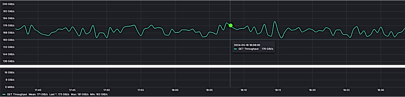
where 16 gateways and 16 DenseIO.E5 storage nodes provide a total sustained 167 GiB/s.
But no, not that kind of “large” we’ll be talking about – a different one. In fact, to demonstrate the distinction I’ll be using my development Precision 5760 (Ubuntu 22, kernel 6.5.0) and running the most minimalistic setup one can only fathom:
a single v3.23.rc4 AIS node on a single SK Hynix 1TB NVMe, with home Wi-Fi (and related magic) to connect to Amazon S3
and that’s it.
When training on a large dataset
Numbers do matter. Google Scholar search for large-scale training datasets returns 3+ million results (and counting). Citing one of those, we find out that, in part:
Language datasets have grown “exponentially by more than 50% per year”, while the growth of image datasets “seems likely to be around 18% to 31% per year <…>
Growth rate notwithstanding, here’s one unavoidable fact: names come first. Training on any dataset, large or small, always begins with finding out the names of contained objects, and then running multiple epochs, whereby each epoch entails computing over a random permutation of the entire dataset – the permutation that, in turn, consists of a great number of properly shuffled groups of object names called batches, etc. etc.
Back to finding out the names though – the step usually referred to as listing objects. The question is: how many. And how long will it take…
What’s in a 10 million names
In the beginning, our newly minted single-node cluster is completely empty – no surprises:
$ ais ls
No buckets in the cluster. Use '--all' option to list matching remote buckets, if any.
But since in aistore accessibility automatically means availability
achieving this equivalency for training (or any other data processing purposes) is a bit tricky and may entail (behind the scenes) synchronizing cluster-level metadata as part of a vanilla read or write operation
– we go ahead to find out what’s currently accessible:
$ ais ls --all
NAME          PRESENT
s3://ais-10M  no
...
Next, we select one bucket (with a promising name) and check it out:
$ ais ls s3://ais-10M --cached --count-only
Listed: 0 names (elapsed 1.27355ms)
Empty bucket it is, aistore wise. What it means is that we’ll be running one exclusively-remote list-objects, with no object metadata coming from the cluster itself.
There’s a balancing act between the need to populate
list-objectsresults with in-cluster metadata, on the one hand, and the motivation not to run N identical requests to remote backend. When aistore has N=1000 nodes, there’ll be still a single randomly chosen target that does the remote call and shares the results with the rest 999.
Listing 10M objects with and without inventory
Frankly, since I already know that top-to-bottom listing of the entire 10-million bucket will require great dedication (and even greater patience), I’ll just go ahead and limit the operation to the first 100K names (that is, 100 next-page requests):
$ for i in {1..10}; do ais ls s3://ais-10M --limit 100_000 --count-only; done

1: 100,000 names in 18.2s
2: 100,000 names in 20.4s
3: 100,000 names in 20.1s
...
And now, for comparison, the same experiments with the new v3.23 feature called bucket inventory. Except that this time – no excuses: we name every single object in the entire 10M dataset (the names are not shown):
$ for i in {1..10}; do ais ls s3://ais-10M --inventory --count-only; done

1. 10,900,489 names in 1m57s
2. 10,900,489 names in 22.94s
3. 10,900,489 names in 22.7s
...
In conclusion – and discounting the first run whereby aistore takes time to update its in-cluster inventory (upon checking its remote existence and last-modified status) – the difference in resulting latency is, roughly, 94 times.
BLOBs
Moving on: from large datasets – to large individual objects. The same persistent question remains: what would be the minimal size that any reasonably unbiased person would recognize as “large”?
Today, the answer will likely fall somewhere in the (1GB, 1PB) range. Further, given some anecdotal evidence – for instance, the fact that Amazon S3 object cannot exceed the “maximum of 5 TB” – we can maybe refine the range accordingly. But it’ll be difficult to narrow it down to, say, one order of magnitude.
A bit of Internet trivia: 1997 USENIX report estimated distribution file types and sizes, with sizes greater than 1MB ostensibly not present at all (or, at least, not discernable in the depicted diagram). And in the year 2000 IBM was publishing special guidelines to overcome 2GB file size limitation.
What I’m going to do now is simply postulate that 1GiB is big enough for at-home experiments
$ ais ls s3://ais-10M --prefix large
NAME      SIZE      CACHED
largeobj  1.00GiB   no
– and immediately proceed to run the second pair of micro-benchmarks:
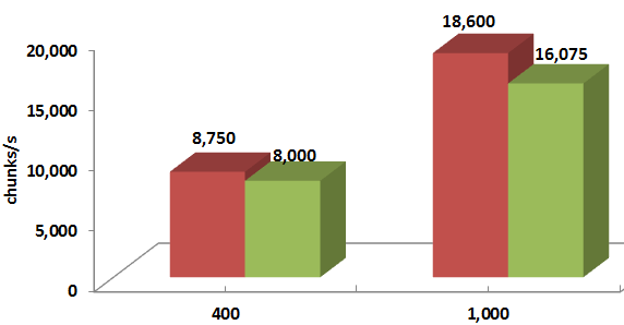
## GET (and immediately evict) a large object
$ for i in {1..10}; do ais get s3://ais-10M/largeobj /dev/null; ais evict s3://ais-10M/largeobj; done
1. 27.4s
2. 27.3s
3. 28.1s
...
versus:
## GET the same object via blob downloader
$ for i in {1..10}; do ais get s3://ais-10M/largeobj /dev/null --blob-download; ais evict s3://ais-10M/largeobj; done
1. 17.4s
2. 16.9s
3. 18.1s
...
The associated capability is called blob downloading – reading large remote content in fixed-size chunks, in parallel. The feature is available in several different ways, including the most basic RESTful GET (above).
Next steps
Given that “large” only gets bigger, more needs to be done. More can be done as well, including both inventory (that can be provided across all remote aistore-supported backends and managed at finer-grained intervals and/or upon events), and blobs (that should be able to leverage the upcoming chunk-friendly content layout). And more.


