Finding the right storage system

What are the odds that you find the right storage system to run all the workloads that need to be running and to forever sustain all the apps that consume storage? Given the current state of the art, what would be your chances of doing so today?

Apart from being existential, the question also appears to be formalizable. Meaning that it can be approached with a certain degree of scientific rigor and scrupulousness. Of course, I’m talking about the Drake equation.

The Drake equation is a probabilistic argument used to estimate the number of active, communicative extraterrestrial civilizations in the Milky Way galaxy. Since its 1961 publication, and notwithstanding constructive criticism (see, for instance,The Drake Equation Is Broken; Here’s How To Fix It“) the equation proved to be usable across wide range of application domains.

Perhaps the most popular application of Drake is estimating one’s chances to find true love (variations: girlfriend, boyfriend, soulmate, BFF).

Given a massive body of work on the subject I’ll have to limit citations to maybe just one: the 2008 paper “Why I don’t have a girlfriend” where Peter Backus clearly and succinctly explains a) how to apply Drake, and b) why at the time of the writing he didn’t have a girlfriend.

Back to storage systems though – equipped with Drake’s methodology, the question of finding the one and only storage system can be factorized (step 1), with the probabilities of each factor estimated (step 2), and fed into the equation (step 3) to generate an estimate. Consider a real-life example, whereby the storage system in question features:

  1. SDS: software stack on commodity x86 servers
  2. Price $0.10/GB or below that covers hardware + software + 5 years of support
  3. Petascale clustering with 1PB usable today and growing to 100PB later in 2019
  4. Storage media: hard drives
  5. Linearity: must scale close to linear with each added node and each added spindle
  6. HA: must be highly available
  7. Tiering: unlimited
  8. Data redundancy: both local (RAID1/5/6/10) and replicated
  9. AI: built-in accelerations for AI workloads

A quick look at the above reveals the truth: the chance of locating a match is probably low.

Indeed, at the time of this writing, the Wikipedia’s computer storage category includes a total of about 150 companies. Even if we super-generously give each of the 9 factors an average 0.5 probability, the resulting (150 * 1/512) can only be interpreted as: oops, doesn’t exist.

There are numerous ways to confirm the first suspicion. For instance, given the limited dataset of 150, we could run Monte Carlo simulations by randomly selecting storage companies and filling-in samples, e.g.:

Storage company X.Y.Z. SDS: No Petascale: No Price: Not cheap Commodity x86: No HA: Yes

Having accumulated enough samples to generate confidence intervals, we then compute the odds, find them depressingly low, and resort to finding some peace in the pure logic of this exercise, a consolation similar to the one Peter Backus found years ago.

We could also take a more conventional route which (conventionally) entails: reviewing datasheets, meeting with vendors, gathering references, reading Top-N IDC and Gartner reports, and then again reviewing the product datasheets. Here, for instance, are the top 13 companies from the IDC Worldwide Object Storage 2018 – we could take this report and painstakingly fill-in a 13-by-9 comparison table with those companies in the rows and the distinguishing characteristics in the columns (I will leave this as an exercise for the reader).

IDC-WOS-2018

Source: The Register

Most likely, though, if nothing even remotely plausible comes up on the first day or two of screening, referencing, and filling out comparison tables, the chance (of finding the right storage system) must be considered extremely slim. The storage system that you need, seek, and depend upon may not exist.

Or, stated differently, the storage system that you really need may really not exist.

It’ll be hard to come to terms with this statement – the process will usually take anywhere between three to nine months. Eventually, though, the dilemma will crystallize as a simple binary choice: to build or not to build?

This is a tough choice to make. Here’s one possible answer. Why does it work for the 9 (nine) factors listed above and where does it go from there – that will be another story and a different time.

Ten Billion Objects and the Pursuit of Balance

Suppose, you’ve come across a set of 10 billion unique objects that are stored far, far away. You can now read them all, although that may at times be painfully slow, if not downright sluggish. And it may be costly as well – a couple cents per gigabyte quickly runs up to real numbers.

You also have a Data Center, or, to be precise, a colocation facility – a COLO. With just a handful of servers, and a promise to get more if things go well. Say, a total of N > 1 servers at your full disposal. The combined capacity of those N servers will not exceed one million objects no matter what – 0.01% of grand total.

Last but not the least, you’ve got yourself a machine-learning project. The project requires each compute job to read anywhere from 100K to 1M random objects out of the 10 billion stored far, far away. The greediest batch job may consume, and then try to digest, close to a million but no more.

Therein lies the question: how to utilize your N-server resource for optimal (i.e., minimal) read latency and optimal (i.e., minimal) outbound transfer cost?

Researching and Developing. Coding.

The reality of R&D is that it’s not like in the movies. It is mundane, repetitive. You tweak and run and un-tweak and rerun. This process can go on and on, for hours and days in a row. Most of the time, though, the job that undergoes the “tweaking” would want to access the same objects.

Which is good. Great, actually, because of the resulting, uneven and unbalanced, distribution of the hot/cold temperatures across the 10-billion dataset. This is good news.

In real life, there are multiple non-deterministic factors that independently collaborate. Running 27 tunable flavors of the same job can quickly help to narrow down the most reusable object set. Impromptu coffee break (factor) presenting a unique opportunity to run all 27 when the rest of the team is out socializing. And so on.

More often, though, it’d be a work-related routine: a leak or a crash, a regression. The one that, down the road, becomes reproducible and gets narrowed to a specific set of objects that causes it to reproduce. The latter then is bound to become very hot very soon.

In pursuit of balance

For whatever reason, the title phrase strongly associates itself with the California pinot noir and chardonnay. There’s the other type of balance though – the one that relates to software engineering. In particular, relates to read caching.

DHT is, maybe, the first thing that comes to mind. The DHT that would be mapping object IDs (OID) to their server locations, helping us to realize the most straightforward implementation of a distributed read cache.

Conceptually, when an object with OID = A shows up in its local server space computing job would execute DHT.insert(A). And then, DHT.delete(A) when a configured LRU/LFU/ARC policy triggers the A’s eviction. The operations would have to be transactional, so that DHT.get() always gets consistent and timely results.

There is a price though. For starters, the task of managing local caches does not appear to be the first concern when all you need is to make your zillion-layer neural network converge (and it wouldn’t).

Thus, the DHT (or whatever is the implementation of the cluster-wide key/value table) would have to be properly offloaded to a separate local daemon and, project-wise, relegated to the remainder of working hours.

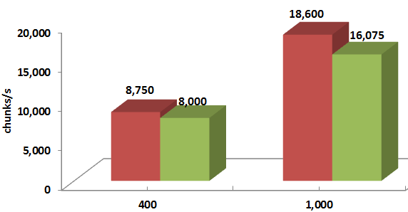
Next, there is a flooding concern. A modest 1K objects-per-second processing rate by 10 concurrent jobs translates as 20K/s inserts and deletes on the DHT. That’s not a lot in terms of bandwidth but that is something in terms of TCP overhead and network efficiency. The control-messaging overhead tends to grow as O(number-of-jobs * number-of-servers) to ultimately affect the latency/throughput of critical flows.

In addition, local DHT daemon will have to discover other DHT daemons and engage them in a meaningful, albeit measured, conversation including (for starters) keep-alive and configuration-change handshakes. So that everyone keeps itself in-sync with everyone else, as far as this (meticulous) object tracking and stuff.

Further, there’s the usual range of distributed scenarios: servers joining and leaving (or crashing, or power-cycling, or upgrading), spurious messaging timeouts, intermittent node failures, inconsistent updates. Think distributed consensus. Think false-positives. Think slipping deadlines and headaches.

And then there is persistence across reboots – but I’ll stop. No need to continue in order to see a simple truth: the read-caching feature can easily blow itself out of all proportions. Where’s the balance here? Where is the glorified equilibrium that hovers in the asymptotic vicinity of optimal impact/effort and cost/benefit ratios? And why, after all, when California pinot noir and chardonnay can be perfectly balanced – why can’t the same be done with software engineering of the most innovative machine-learning project that simply wants to access its fair share of objects stored far, far away?

The pause

The idea is as old as time: trade distributed state for distributed communications, or a good heuristic, or both. Better, both.

Hence, it’d be very appropriate at this point to take a pause and observe. Look for patterns, for things that change in predictable ways, or maybe do not change at all…pob-pause

When object sets are static

It appears that many times the compute jobs would know the contents of their respective object sets before their respective runtimes. Moreover, those objsets can be totally preordered: an object B would follow an object A iff the B is processed after the A, or in parallel.

The phenomenon can be attributed to multiple runs and reruns (previous section) when all we do is update the model and see if that works. Or, it can be ascribed to searchable metadata that happens to be stored separately for better/faster observability and analytics. Whatever the reason, the per-job list of object IDs can be compiled and broadcast to the clustered servers, accompanied with the message to please hold-on to those objects if they are local.

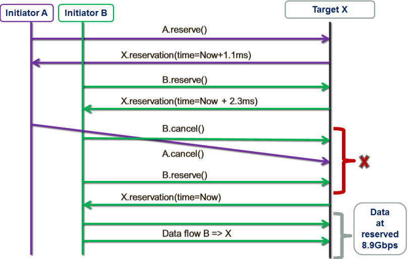
More precisely, the steps are:

  1. A job that is about to start executing broadcasts the list of its OIDs as well as per-OID (min, max, location) records of when and where it’ll need the objects preloaded;
  2. Each of the (N-1) control plane daemons responds back with a message consisting of a bunch of (OID, t1, t2) tuples, where OID is an object ID and:
    • t1 = 0, t2 > 0: the object is local at the responding server, and the server commits to keep it until at least time = t2
    • t1 > 0, t2 > t1: the object is not currently present at the responding server; the server, however, makes a tentative suggestion (a bid) to load it by the time t1 and keep it until the time t2
  3. Finally, the job collects all the responses and in turn responds back to all the bids canceling some of them and confirming the others.

So that’s that – the fairly straightforward 3-step procedure that converges in seconds or less. There are, of course, numerous and fine details. Like, for instance, how do we come up with the t1 and t2 estimates to balance the load of already started or starting jobs while not degrading the performance of those that may come up in the future. Or the question of how to optimally calibrate the bidding process at runtime. And so on.

Those are the types of details that are beyond the point of this specific text. The point is, utilize both the prior knowledge and the combined N-server resource. Utilize both to the maximum.

When object sets are dynamic

But what if the object sets are not static, as in:pod-next-oidCould we still optimize when the next object is not known until the very last moment it needs to be processed? Clearly, the problem immediately gets infinitely trickier. But not all hope is lost if we take another pause…pob-pause

– to experiment a bit and observe the picture:

pob-virtsnap

Fig 1. Percentage of virtually snapshotted objects as a function of elapsed time.

No, this is not an eternal inflation of the multiverse with bubble nucleation via quantum tunneling. This is a tail distribution aka CCDF – the percentage of objects that remain local after a given interval of time – a cluster-wide survival function. To obtain that curve, a simple script would visit each server node and append its local object IDs to a timestamped log, in effect creating a virtual snapshot of the clustered objects at a given time.

Later, the same script uses the same log to periodically check on the (virtually snapshotted) objects. In the Fig. 1, the bump towards the end indicates reuploading of already evicted objects – the fact that strongly indicates suboptimal behavior of the system. Subsequently, after factoring-in environmental differences and gaussian noise (both causing the shape of CCDF to falter and flap across job runs and coffee breaks), we obtain this:

pob-survival

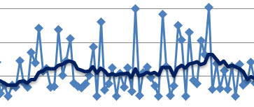
Fig 2. Survival function with noise

One observation that stands strong throughout the experiments is that an object almost never gets evicted during the first time talive interval of its existence inside the compute cluster. As time goes by, the chances to locate most of the original virtual snapshot in the cluster slowly but surely approach zero depicted as a fuzzy reddish area at the bottom of the Fig. 2.

The fork

Clearly, for any insight on the dynamic object locations, we need to have some form of virtual snapshotting. Introduce it as a cluster-wide periodic function, run it on every clustered node, broadcast the resulting compressed logs, etc.

But how often do we run it? Given an observed average lifecycle of a virtual snapshot T (Fig. 2), we could run it quite frequently – say, every max(T/10,000, 1min) time, to continuously maintain an almost precise picture of object locations (all 10 billion of those).

Alternatively, we could run it infrequently – say, every min(T/2, talive) – and derive the corresponding P(is-local) probabilities out of the approximated survival function.

Hence, the dilemma. The fork in the road.pob-pause

Bernoulli

Since the “frequent” option is a no-brainer (and a costly one), let’s consider the “infrequent” option first, with the intention to make it slightly more frequent in the future, thus approximating the ultimate optimally-balanced compromise. Given an object’s OID and bunch of outdated virtual snapshots, we should be able to track the object to the last known time it was uploaded from far, far away. Let’s call this time toid:

pob-bernoulli

Fig 3. Bernoulli trial

Next, notice that for any two objects A and B, and a sufficiently small interval dt the following would hold:pob-a-and-b-localThat is, because the objects that have similar local lifetimes within the compute cluster must also have similar chances of survival.

Further, select a sufficiently small dt (e.g., dt = (T – talive – tdead)/100) and, when a job starts executing, gradually gather an evidence denoted in the Fig. 3 as yes and no for: “object is local” and “not local”, respectively. Each small interval then automatically becomes an independent Bernoulli trial with its associated (and yet unknown) probability p(dt) and the Binomial PMF:pob-binomial-pmfThe question is how we can estimate the p for each or some of the 100 (or, configured number of) small intervals. One way to do it is via Bayesian posterior update that takes in two things:

  1. the prior probability p, and
  2. the Bernoulli trial evidence expressed as two integers: n (number of objects) and k (number of local objects),

and transforms all of the above into the posterior probability distribution function:pob-beta-distributionHere’s how this formula is working out. Recall that n and k are two counters that are being measured on a per dt basis. On the right side of the equation, we have the Bayes’ theorem that divides the prior probability (of k successes in the n Bernoulli trials) by the total probability (of k successes in the n Bernoulli trials). The prior in this case corresponds to our belief that the real probability equals p.

On the left side, therefore, is a posterior probability distribution function parametrized by p – a formula of the most basic type y = f(x) which can be further used to estimate the expected value and its variance, integrate across intervals (to approximate parts of the CDF), and so on.

Wrapping up

The  formula above happens to be the standard Beta distribution. Which means that from gathering per-interval statistics to estimating per-interval probabilities, there is a single step that sounds as follows: go ahead and look up the corresponding Wikipedia page. Arguably, that step can be performed just once, maybe two or (max) three times.

That helps. What helps even more is the general downtrend of the survival functions, from which one can deduce that “giving up” on finding the objects locally for a certain specific interval (ti, ti + dt) can be followed by abandoning ongoing efforts (if any) to compute the probabilities to the right of this ti.

Further, the notion of “giving up” vs “not giving up” will have to be defined as a threshold probability that is itself a function of the cumulative overhead of finding the objects locally, normalized by the number of successful finds.

However. It is incumbent upon us to wrap it up. Other fascinating details pertaining to the business of handling treasure troves of billions, trillions, and Graham numbers of objects will have to wait until they can be properly disclosed.

All in due time.

Choosy Initiator

In a fully distributed storage cluster (FDSC), one possible design choice for a new storage protocol is resource reservation (RR). There are certain distinct challenges though, when working out an optimal RR schema. On the storage initiator side, one critical question that arises is whether to accept an RR response a.k.a. a bid from a given target for a given I/O request. Or, alternatively, try to renegotiate, in hopes of getting a better reservation.

The absolutely best reservation is, of course, the one that allows I/O in question to start immediately and execute at full throttle.

Hence, choosy initiator in the title, the storage initiator that grapples with the dilemma: go ahead and accept possibly suboptimal arrangement, or renegotiate. The latter inevitably comes with the risk to receive future reservations that are even more delayed.

To bet or not to bet, that is the question. To find out, I’ve used SURGE: a discrete open source event simulation framework written in Go (https://golang.org/doc/). The source includes a bunch of concrete protocol models (that run) and the usual README to get started.

OK, let’s do some definitions.

FDSC and RR

The three key aspects of a FDSC are self-containment, full connectivity, and hashed distribution:

  • Self-containment: each clustered node is a sole owner of its local resources: disks, CPU, memory, and link bandwidth;
  • Any-to-any: all nodes are interconnected through non-blocking, no-drop network core;
  • Hashed memoryless distribution: a given I/O request is mapped or hashed to a number of storage target. For writes, the number of targets must be equal or greater than the required redundancy. This I/O mapping/hashing operation does not depend on the history and on any of the previously executed I/O requests (hence, memoryless).

Note separately that the letter ‘S’ in FDSC also reads as “symmetric”. In symmetric clusters, each node performs a dual role of storage initiator and storage target simultaneously.

For now let’s just say that large fully distributed clusters counting hundreds or thousands initiators and targets require a different intra-cluster transport. That’s #1, the point that maybe does not sound very controversial. To add controversy (just for the heck of it), here’s the point #2: for large and super-large FDSC it makes a lot of sense to use RR based transport protocols. One of the key proof points boils down to convergence.

Convergence time is the time it takes for existing link-sharing (path-sharing) flows to converge on their respective optimal rates when a new flow is being added or an existing flow removed. All things being equal, each of the N flows eventually must take 1/Nth of the total bandwidth.

Figure 12 in the research paper at http://goo.gl/JUlijH shows DCTCP convergence times.

Red flow (below) is added after the blue flow has reached its steady and close-to-optimal state. The research estimates DCTCP convergence times on a 10GE network ranging anywhere from 229*d to 770*d, where d is the propagation delay. This is a considerable time corresponding to several fully transferred 128K payloads even for a very favorable (as far as speedy convergence) value of d in the order of few microseconds.

choosy-fig1
Figure 1. DCTCP convergence (courtesy DCTCP research)

In presence of multiple flows the picture gets substantially more messy but the bigger point is: irrespective of the particular link-sharing transport, during the time N flows are converging from (N-1) or (N+1), they all execute at sub-optimal rates resulting in overall sub-optimal network utilization. Hence, an appeal of the RR approach: eliminate resource sharing. Utilization time slots are simply negotiated. There will be no unexpected start-IO, complete-IO, and add-flow, delete-flow events in the middle.

If there exists anything similar in real life, that could be a timeshare ownership. On the networking side examples include RSVP in its unicast and multicast realizations (RFC2205).

In all cases (including timeshare) and independently of the concrete resource reservation protocol, each successful RR negotiation comes with a time window in combination with a full set of requested targets resources – for exclusive usage (during a given time window) by a given pending request (emphasis on exclusive). For each I/O request, there is a natural progression:

I/O request =>
   potential targets =>
      RR negotiation(s) =>
          data flows to/from ...

This results in network flows executing as prescribed by non-overlapping time windows granted in turn by the respective selected targets.

To bet or not to bet

The figure below shows one possible “resource reservation, renegotiated” (RRR) scenario:

choosy-fig2
Figure 2. RRR (example)

There are two storage initiators: purple A and green B. The initiators are trying to establish data flows with the same target X at approximately the same time.

First, initiator A tentatively reserves target X for a window starting 1.1ms later (from now), which roughly corresponds to the time target X needs to complete a (presumably) already queued 1MB transaction (not shown here).

Next, initiator B tentatively reserves X for the adjacent X’s time window at 2.3ms from now. Red X on the picture indicates the decision point.

In this example, instead of accepting whatever is presented to it at the moment, B decides that 2.3ms is too much of a delay and cancels. Simultaneously, A cancels as well, possibly because it has obtained more attractive bids from other storage targets that are not shown here. This further results in B getting the optimal reservation and utilizing it right away.

Simulation

The idea that at least sometimes it does make sense to take a risk and renegotiate requires proof. Fortunately, with SURGE we can run massive simulations to find out.

Replicast is a one FDSC-friendly RR-based protocol that was previously described – see for instance SNIA presentation Beyond Consistent Hashing and TCP.

Replicast-H (where H stands for hybrid) entails multicast control plane and unicast data. Recall that RR negotiation is a part of the reservations-based protocol control plane. When running a hybrid version of the Replicast, we negotiate up to (typically) 3 successive time windows to perform a write. We then often see the following picture:

choosy-fig3

Figure 3. Reservations without renegotiation

This above is a 200-point random sample that details latencies of 1MB size chunks written into their hashed target destinations. Green trendline in the middle shows 10-point moving average. This is a “plain” Replicast-H benchmark where each target’s bid is taken at a face value and never renegotiated.

The cluster in this case combines 90 targets and 90 storage initiators with targets operating at 1000MB/s disk throughput. Finally, there is a non-blocking no-drop 10Gbps that connects each target with each initiator.

In the simulation above 10% of the bandwidth is statically allocated for control traffic. With 1% accounting for network headers and miscellaneous overhead, that leaves 8.9Gbps for (pure) data.

In the idealistic conditions when a given initiator does not have any competition from others, the times to execute a 1MB write to a single target would be, precisely:

  • Network: 941.482µs
  • Disk: 1ms

Given 3 copies, the request could (ideally) be fully executed in slightly more than 4 milliseconds, including control handshakes and acknowledgements.

There is, however, inevitably a competition resulting in reservation conflicts and delays, and further manifesting itself in occasional end-to-end spikes up to 7ms latency and beyond – see the picture above.

In depth analysis of traces (that I will skip here) indicates that, indeed, one possible reason for the spikes is that initiators accept reservations too early. For instance, the initiator that executed the #5 in the sample (Fig. 3) could likely do better.

Unicast delivery with renegotiation

This “with renegotiation” flavor of the protocol adds a new configuration variable that currently defaults to 3 times RTT on the control plane:

choosy-fig-code1

Note: to go directly to the github source, click this and other similar code fragments. At runtime, this model will double the wait time and renegotiate reservations if and when the actual waiting time (denoted as ‘idletime’ below) exceeds the current value:

choosy-fig-code4

In addition, since 3 times RTT is just a crude initial guess, each modeled gateway (a.k.a. storage initiator) recomputes its value (‘r.maxbidwait’ in the code) for the next write request, averaging the previous value and the current one:

choosy-fig-code3

What happens after the first few transactions is that each initiator independently computes an objective average delay and from there on renegotiates only when the newly collected reservations collectively result in substantially bigger delay (in other words, the initiator renegotiates only when it “thinks” it could get a better deal).

Here’s the SURGE-simulated result for apples-to-apples identical configuration that runs 90 storage initiators and 90 storage targets, etc.:

choosy-fig4
Figure 4. Reservations with renegotiation

Notice that there are no 7ms spikes anymore. They are simply gone.

Conclusions, briefly

For differently sized chunks and disk/backend throughputs, the average improvement ranges from 8% to 20%:

choosy-fig5
Figure 5. 128K chunks, 400MB/s disk (left) and 1000MB/s disk (right)

Legend-wise, red columns depict the “with renegotiation” version.

choosy-fig6
Figure 6. 1MB chunks, 400MB/s disk (left) and 1000MB/s disk (right)

Thus, taking a risk does seem to pay off: RR based protocol where storage initiators are “choosy” and at least sometimes renegotiate their reservations outperforms its prior version.

SURGE: performance modeling for distributed systems

Foreword

As far as distributed system and storage software, finding out how it'll perform at scale - is hard.

Expensive and time-consuming as well, often impossible. When there are the first bits to run, then there’s maybe one, two hypervisors at best (more likely one though). That’s a start.

Early stages have their own exhilarating freshness. Survival is what matters then, what matters always. Questions in re hypothetical performance at 10x scales sound far-fetched, almost superficial. Answers are readily produced – in flashy powerpoints. The risk however remains, carved deep into the growing codebase, deeper inside the birthmarks of the original conception. Risk that the stuff we’ll spend next two, three years to stabilize will not perform.

The Goal

The goal is modeling the performance of a distributed system of any size (emphasis on modeling, performance and any size). Which means – uncovering the behavioral patterns (periodic spike-downs and, generally, any types of pseudo-regular irregularities), charting throughputs and latencies and their respective distributions concealed behind performance averages. And tails of those distributions, those that are in the single-digit percentile ranges.

Average throughput, average IOPS, average utilization, average-anything is not enough – we need to see what is really going on. For any scale, any configuration, any ratios of: clients and clustered nodes, network bandwidth and disk throughput, chunk/block sizes, you name it.

Enter SURGE, discrete event simulation framework written in Go and posted on GitHub. SURGE translates (admittedly, with a certain effort) as Simulator for Unsolicited and Reservation Group based and Edge-driven distributed systems. Take it or leave it (I just like the name).

Go aka golang, on the other hand, is a programming language1 2.

Go

Go is an open source programming language introduced in 2007 by Rob Pike et al. (Google). It is a compiled, statically typed language in the tradition of C with garbage collection, runtime reflection and CSP-style concurrent programming.

CSP stands for Communicating Sequential Processes, a formal language, or more exactly, a notation that allows to formally specify interactions between concurrent processes. CSP has a history of impacting designs of programming languages.

Runtime reflection is the capability to examine and modify the program’s own structure and behavior at runtime.

Go’s reflection appears to be very handy when it comes to supporting IO pipeline abstractions, for example. But more about that later. As far as concurrency, Rob Pike’s presentation is brief and to the point imho. To demonstrate the powers (and get the taste), let’s look at a couple lines of code:

play.golang.org/p/B7U_ua0bzk

In this case, notation 'go function-name' causes the named function to run in a separate goroutine – a lightweight thread and, simultaneously, a built-in language primitive.

Go runtime scheduler multiplexes potentially hundreds of thousands of goroutines onto underlying OS threads.

The example above creates a bidirectional channel called messages (think of it as a typed Unix pipe) and spawns two concurrent goroutines: send() and recv(). The latter run, possibly on different processor cores, and use the channel messages to communicate. The sender sends random ASCII codes on the channel, the receiver prints them upon reception. When 10 seconds are up, the main goroutine (the one that runs main()) closes the channel and exits, thus closing the child goroutines as well.

Although minimal and simplified, this example tries to indicate that one can maybe use Go to build an event-distributing, event-driven system with an arbitrary number of any-to-any interconnected and concurrently communicating players (aka actors). The system where each autonomous player would be running its own compartmentalized piece of event handling logic.

Hold on to this visual. In the next section: the meaning of Time.

Time

In SURGE every node of a modeled cluster runs in a separate goroutine. When things run in parallel there is generally a need to go extra length to synchronize and sequence them. In physical world the sequencing, at least in part, is done for us by the laws of physics. Node A sending message to remote node B can rest assured that it will not see the response from node B prior to this sent message being actually delivered, received, processed, response created, and in turn delivered to A.

The corresponding interval of time depends on the network bandwidth, rate of the A ⇔ B flow at the time, size of the aforementioned message, and a few other utterly material factors.

That’s in the physical world. Simulated clusters and distributed models cannot rely on natural sequencing of events. With no sequencing there is no progression of time. With no progression there is no Time at all – unless…

Unless we model it. For starters let’s recall an age-old wisdom: time is not continuous (as well as, reportedly, space). Time rather is a sequence of discrete NOWs: one indivisible tick (of time) at a time. Per quantum physics the smallest time unit could be the Planck time ≈5.39*10-44s although nobody knows for sure. In modeling, however, one can reasonably ascertain that there is a total uneventful void, literally nothing between NOW and NOW + 1.

In SURGE, the smallest indivisible tick of time is 1 nanosecond, a configurable default.

In a running operating physical cluster each NOW instant is filled with events: messages ready to be sent, messages ready to be received, events being handled right NOW. There are also en route messages and events sitting in disk and network queues and waiting for their respective future NOWs.

Let’s for instance imagine that node A is precisely NOW ready to transmit a 8KB packet to node B:

node-a-to-node-b

Given full 10Gbps of unimpeded bandwidth between A and B and the trip time, say, 1µs, we can then with a high level of accuracy predict that B will receive this packet (819ns + 1µs) later, that is at NOW+1.819µs as per the following:

play.golang.org/p/RZpYY_hNnQ

In this snippet of modifiable-and-runnable code, the local variable sizebits holds the number of bits to send or receive while bwbitss is a link bandwidth, in bits per second.

Time as Categorical Imperative

Here’s a statement of correctness that, on the face of it, may sound trivial. At any point in time all past events executed in a given model are either already fully handled and done or are being processed right now.

A past event is of course an event scheduled to trigger (to happen) in the past: at (NOW-1) or earlier. This statement above in a round-about way defines the ticking living time:

At any instant of time all past events did already trigger.

And the collateral:

Simulated distributed system transitions from (NOW-1) to NOW if and only when absolutely all past events in the system did happen.

Notice that so far this is all about the past – the modeled before. The after is easier to grasp:

For each instant of time all future events in the model are not yet handled - they are effectively invisible as far as designated future handlers.

In other words, everything that happens in a modeled world is a result of prior events, and the result of everything-that-happens is: new events. Event timings define the progression of Time itself. The Time in turn is a categorical imperative – a binding constraint (as per the true statements above) on all events in the model at all times, and therefore on all event-producing, event-handling active players – the players that execute their own code autonomously and in parallel.

Timed Event

To recap. Distributed cluster is a bunch of interconnected nodes (it always is). Each node is an active Go player in the sense that it runs its own typed logic in its own personal goroutine. Nodes continuously generate events, assign them their respective computed times-to-trigger and fan them out onto respective Go channels. Nodes also continuously handle events when the time is right.

By way of a sneak peek preview of timed events and event-driven times, here’s a life of a chunk (a block of object’s data or metadata) in one of the SURGE’s models:
example-executed-chunk
The time above runs on the left, event names are abbreviated and capitalized (e.g. MCPRE). With hundreds and thousands of very chatty nodes in the model, logs like this one become really crowded really fast.

In SURGE framework each and every event is timed, and each timed event implements the following abstract interface:

type EventInterface interface {
    GetSource() RunnerInterface
    GetCreationTime() time.Time
    GetTriggerTime() time.Time
    GetTarget() RunnerInterface
    GetTio() *Tio
    GetGroup() GroupInterface
    GetSize() int
    IsMcast() bool
    GetTioStage() string
    String() string
}

This reads as follows. There is always an event source, event creation time and event trigger time. Some events have a single remote target, others are targeting a group (of targets). Event’s source and event’s target(s) are in turn clustered nodes themselves that implement (RunnerInterface).

All events are delivered to their respective targets at prescribed time, as per the GetTriggerTime() event’s accessor. The Time-defining imperative (above) is enforced with each and every tick of time.

In the next installment of SURGE series: ping-pong model, rate bucket abstraction, IO pipeline and more.

Embracing and Abandoning ZFS

If you are not familiar with ZFS, you should be. It is the best local file system ever developed.

It’s also likely to retain that title forever, because improving the local file system is not where the storage industry’s head is at these days. Distributed storage is the only way to scale-out to the degree that  storage now requires.

My first design for Object Storage at Nexenta sought to leverage ZFS as one implementation of a “Local File System” superclass. It could bring benefits to both our Object Storage clusgter and to OpenStack Swift.  This was a natural progression with evolutionary design. Nexenta is a ZFS company and we were very familiar with ZFS. We wanted to take advantage of the protection provided by ZFS within one server with distributed data protection. We dubbed this the “2+2” strategy. I presented the idea at the OpenStack Folsom summit.

The key advantage that ZFS enabled was the aibity to mix local replication with network replication, as summarized by the following two slides from that presentation:

OpenStackCCOW4 OpenStackCCOW5

The obstacles to this approach proved to be too high. Relying on two network replicas where each machine keeps a high reliability mirror (“2 by 2”) can only achieve the same availability if you have two network ports on each storage server. Without dual network ports the loss of a single network interface leaves you only a single failure from losing access to data.

But dual ports are a concept that virtualization management simply does not want to understand. It wants a single Ethernet link to a single storage node. They either work as a complete unit, or they do not. A “2×2” solution requires tracking nodes that are in “limping” states such as knowing when a storage node is only reachable by one of its two links. Keeping track of the state of each server as being either “working”, “limping” or “dead” sound simple enough, but just “working” or “dead” is a lot simpler. There are other conditions that can put a storage device in a “limping” state where it can be read but should not be written to, such as a drive that is starting to fail. But this is the only thing that would require the management plane to add this concept.

Management plane developers hate adding more concepts when 90% of the world is happy without the additional work. So that wasn’t going anywhere.

We also realized that multicast UDP was a much better solution. Rather than battling to get network management improved so that we could go from 2 excess deliveries to 1 excess delivery we could just use multicast UDP and end up with 0 excess deliveries.

All of these issues were actually minor compared to the challenges of providing high performance object storage using Python.

Basically, it does not work.

Swift advocates will claim otherwise, but they are trying to con you that Object Storage should not be expected to be as high performance as SAN or NAS storage. I don’t buy that line of thinking.

There were several new ideas that we wanted to incorporate in the design, all of which will be covered in later blogs.

  • Totally decentralized control and namespaces.
  • Using multicast communications rather than point-to-point protocols such as TCP/IP.
  • Avoiding the constraints of Consistent Hashing.
  • Truly embracing Key/Value storage, top-to-bottom.

But there were also a lot that we wanted to inherit from ZFS – building upon ideas sometimes works better than directly reusing the code via modularized or layered architectures. Those eternal ZFS ideas, or at least some of them, are:

  • Copy-on-Write: never overwrite in-use data
  • Never Trust Storage Devices
  • Always be Consistent on Disk
  • Use Transaction Logs to Improve Performance
  • Use Snapshots and Clones
  • Replication Is Important
  • "Rampant Layering Violation"

Copy-on-Write

ZFS never overwrites in-use data. It writes new data, and then references the new data. The new object storage system would end up taking this even farther. Each new chunk has its content written exactly once. It can be replicated as needed, but a chunk once written is never updated.

Never Trust Storage Devices

It is not enough to respond to errors when disks report them. You need to validate the data read versus checksums stored elsewhere.

The new object storage system uses cryptographic hashes of each chunk’s payload to identify, locate and validate each chunk.

Always Be Consistent on Disk

The easiest way to always be consistent on what is written to persistent storage is to never write any data which a later action can invalidate.

The CCOW (Cloud Copy-on-Write) object storage system does not rely on any information stored about any chunk other than its cryptographic hash identifier.

Use Transaction Logs to Improve Performance

ZFS relies upon transaction logs to maintain its “always consistent on disk” goal.  The data on disk is consistent, after you apply the pending transactions in the log after a sudden reboot. Updating the root after every transaction is the only other way to always be consistent on disk, and that would require far too many disk writes.

NexentaEdge uses the same technique to allow eventual update of related data structures after a new Version Manifest is written. It cuts the number of disk writes required before an acknowledgement of a Version Manifest Put transaction nearly in half.

Use Snapshots and Clones

ZFS creates snapshots by not deleting them. It can turn them into clones by simply allowing new version forks to branch from there.

Keeping this with a distributed object system was a challenge, but we came up with a method of truly snapshotting a distributed set of metadata. To push the photo analogy it is a true snapshot that captures the system state at one instant, it just needs to be developed before you can see the picture. I’ll describe that in a later blog.

Replication Is Important

How a system replicates data after it is put is not an afterthought. ZFS features snapshot driven replication. That feature is retained by NexentaEdge, just using NexentaEdge snapshots instead.

“Rampant Layering Violation”

Perhaps the most important lesson is an inherited attitude.

ZFS was accused of being a “Rampant Layering Violation”. Jeff Bonwick’s response (https://blogs.oracle.com/bonwick/entry/rampant_layering_violation) was that it was merely more intelligent layering that picked more effective divisions of responsibilities.

NexentaEdge will likely be accused of far worse layering violations.

  • The Replicast protocol considers storage distribution and network utilization at the same time.
  • Since the end user ultimately pays for both we see nothing wrong with optimizing both of them.
  • This is still layered – we only optimize traffic on the storage network. It is physically or logically (VLAN) separated from other networking. Optimizing the storage network for storage is just common sense.

Embracing by Abandoning

NexentaEdge storage servers use key value storage, whether physical or a software simulation of key/value storage. This is the simplest API for copy-on-write storage to use. While it might have been possible to define a key/value ZVol it just isn’t worth the effort. There is too little left of single machine ZFS left to make it worth building NexentaEdge on top of ZFS.

The ideas of ZFS, however, inspired the entire design effort.