SURGE: performance modeling for distributed systems

Foreword

As far as distributed system and storage software, finding out how it'll perform at scale - is hard.

Expensive and time-consuming as well, often impossible. When there are the first bits to run, then there’s maybe one, two hypervisors at best (more likely one though). That’s a start.

Early stages have their own exhilarating freshness. Survival is what matters then, what matters always. Questions in re hypothetical performance at 10x scales sound far-fetched, almost superficial. Answers are readily produced – in flashy powerpoints. The risk however remains, carved deep into the growing codebase, deeper inside the birthmarks of the original conception. Risk that the stuff we’ll spend next two, three years to stabilize will not perform.

The Goal

The goal is modeling the performance of a distributed system of any size (emphasis on modeling, performance and any size). Which means – uncovering the behavioral patterns (periodic spike-downs and, generally, any types of pseudo-regular irregularities), charting throughputs and latencies and their respective distributions concealed behind performance averages. And tails of those distributions, those that are in the single-digit percentile ranges.

Average throughput, average IOPS, average utilization, average-anything is not enough – we need to see what is really going on. For any scale, any configuration, any ratios of: clients and clustered nodes, network bandwidth and disk throughput, chunk/block sizes, you name it.

Enter SURGE, discrete event simulation framework written in Go and posted on GitHub. SURGE translates (admittedly, with a certain effort) as Simulator for Unsolicited and Reservation Group based and Edge-driven distributed systems. Take it or leave it (I just like the name).

Go aka golang, on the other hand, is a programming language1 2.

Go

Go is an open source programming language introduced in 2007 by Rob Pike et al. (Google). It is a compiled, statically typed language in the tradition of C with garbage collection, runtime reflection and CSP-style concurrent programming.

CSP stands for Communicating Sequential Processes, a formal language, or more exactly, a notation that allows to formally specify interactions between concurrent processes. CSP has a history of impacting designs of programming languages.

Runtime reflection is the capability to examine and modify the program’s own structure and behavior at runtime.

Go’s reflection appears to be very handy when it comes to supporting IO pipeline abstractions, for example. But more about that later. As far as concurrency, Rob Pike’s presentation is brief and to the point imho. To demonstrate the powers (and get the taste), let’s look at a couple lines of code:

play.golang.org/p/B7U_ua0bzk

In this case, notation 'go function-name' causes the named function to run in a separate goroutine – a lightweight thread and, simultaneously, a built-in language primitive.

Go runtime scheduler multiplexes potentially hundreds of thousands of goroutines onto underlying OS threads.

The example above creates a bidirectional channel called messages (think of it as a typed Unix pipe) and spawns two concurrent goroutines: send() and recv(). The latter run, possibly on different processor cores, and use the channel messages to communicate. The sender sends random ASCII codes on the channel, the receiver prints them upon reception. When 10 seconds are up, the main goroutine (the one that runs main()) closes the channel and exits, thus closing the child goroutines as well.

Although minimal and simplified, this example tries to indicate that one can maybe use Go to build an event-distributing, event-driven system with an arbitrary number of any-to-any interconnected and concurrently communicating players (aka actors). The system where each autonomous player would be running its own compartmentalized piece of event handling logic.

Hold on to this visual. In the next section: the meaning of Time.

Time

In SURGE every node of a modeled cluster runs in a separate goroutine. When things run in parallel there is generally a need to go extra length to synchronize and sequence them. In physical world the sequencing, at least in part, is done for us by the laws of physics. Node A sending message to remote node B can rest assured that it will not see the response from node B prior to this sent message being actually delivered, received, processed, response created, and in turn delivered to A.

The corresponding interval of time depends on the network bandwidth, rate of the A ⇔ B flow at the time, size of the aforementioned message, and a few other utterly material factors.

That’s in the physical world. Simulated clusters and distributed models cannot rely on natural sequencing of events. With no sequencing there is no progression of time. With no progression there is no Time at all – unless…

Unless we model it. For starters let’s recall an age-old wisdom: time is not continuous (as well as, reportedly, space). Time rather is a sequence of discrete NOWs: one indivisible tick (of time) at a time. Per quantum physics the smallest time unit could be the Planck time ≈5.39*10-44s although nobody knows for sure. In modeling, however, one can reasonably ascertain that there is a total uneventful void, literally nothing between NOW and NOW + 1.

In SURGE, the smallest indivisible tick of time is 1 nanosecond, a configurable default.

In a running operating physical cluster each NOW instant is filled with events: messages ready to be sent, messages ready to be received, events being handled right NOW. There are also en route messages and events sitting in disk and network queues and waiting for their respective future NOWs.

Let’s for instance imagine that node A is precisely NOW ready to transmit a 8KB packet to node B:

node-a-to-node-b

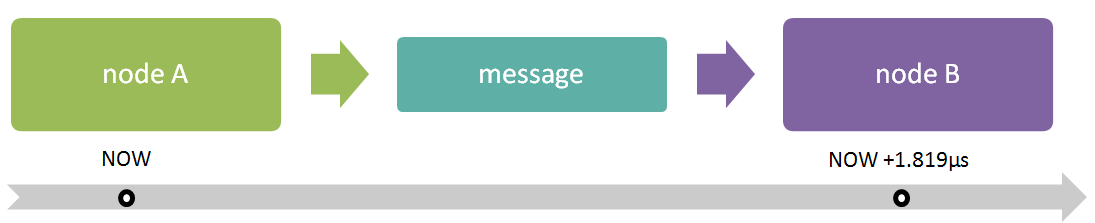
Given full 10Gbps of unimpeded bandwidth between A and B and the trip time, say, 1µs, we can then with a high level of accuracy predict that B will receive this packet (819ns + 1µs) later, that is at NOW+1.819µs as per the following:

play.golang.org/p/RZpYY_hNnQ

In this snippet of modifiable-and-runnable code, the local variable sizebits holds the number of bits to send or receive while bwbitss is a link bandwidth, in bits per second.

Time as Categorical Imperative

Here’s a statement of correctness that, on the face of it, may sound trivial. At any point in time all past events executed in a given model are either already fully handled and done or are being processed right now.

A past event is of course an event scheduled to trigger (to happen) in the past: at (NOW-1) or earlier. This statement above in a round-about way defines the ticking living time:

At any instant of time all past events did already trigger.

And the collateral:

Simulated distributed system transitions from (NOW-1) to NOW if and only when absolutely all past events in the system did happen.

Notice that so far this is all about the past – the modeled before. The after is easier to grasp:

For each instant of time all future events in the model are not yet handled - they are effectively invisible as far as designated future handlers.

In other words, everything that happens in a modeled world is a result of prior events, and the result of everything-that-happens is: new events. Event timings define the progression of Time itself. The Time in turn is a categorical imperative – a binding constraint (as per the true statements above) on all events in the model at all times, and therefore on all event-producing, event-handling active players – the players that execute their own code autonomously and in parallel.

Timed Event

To recap. Distributed cluster is a bunch of interconnected nodes (it always is). Each node is an active Go player in the sense that it runs its own typed logic in its own personal goroutine. Nodes continuously generate events, assign them their respective computed times-to-trigger and fan them out onto respective Go channels. Nodes also continuously handle events when the time is right.

By way of a sneak peek preview of timed events and event-driven times, here’s a life of a chunk (a block of object’s data or metadata) in one of the SURGE’s models:
example-executed-chunk
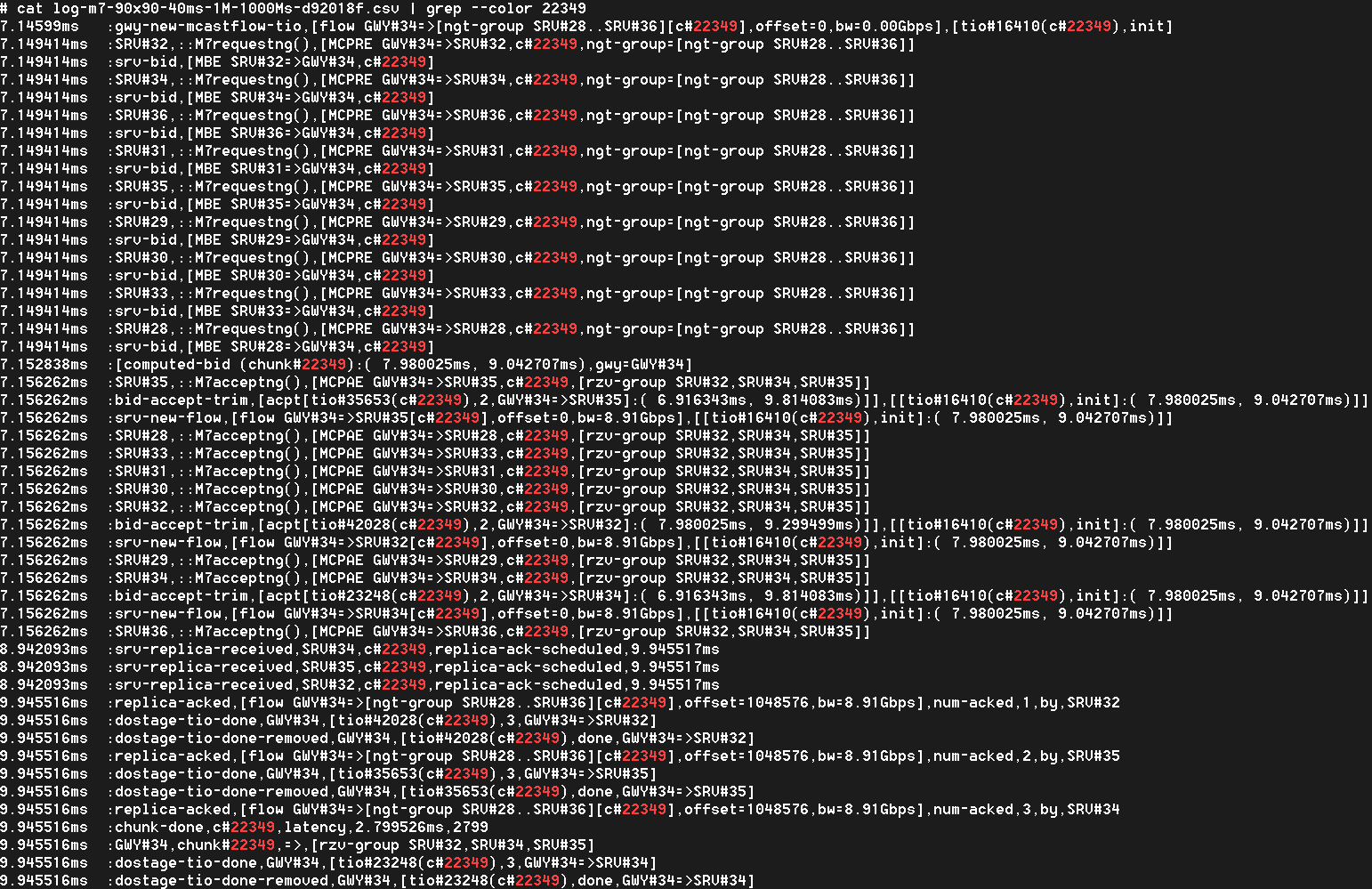
The time above runs on the left, event names are abbreviated and capitalized (e.g. MCPRE). With hundreds and thousands of very chatty nodes in the model, logs like this one become really crowded really fast.

In SURGE framework each and every event is timed, and each timed event implements the following abstract interface:

type EventInterface interface {
    GetSource() RunnerInterface
    GetCreationTime() time.Time
    GetTriggerTime() time.Time
    GetTarget() RunnerInterface
    GetTio() *Tio
    GetGroup() GroupInterface
    GetSize() int
    IsMcast() bool
    GetTioStage() string
    String() string
}

This reads as follows. There is always an event source, event creation time and event trigger time. Some events have a single remote target, others are targeting a group (of targets). Event’s source and event’s target(s) are in turn clustered nodes themselves that implement (RunnerInterface).

All events are delivered to their respective targets at prescribed time, as per the GetTriggerTime() event’s accessor. The Time-defining imperative (above) is enforced with each and every tick of time.

In the next installment of SURGE series: ping-pong model, rate bucket abstraction, IO pipeline and more.

Hyperconvergence: the Litmus Test

What’s in the name

It is difficult to say when exactly the “hyper” prefix was the first time attached to “converged” infrastructure. Hyper-convergence, also known as hyperconvergence, ultimately means a fairly simple thing: running user VMs on virtualized and clustered storage appliances. The latter in turn collaborate behind the scenes to a) pool combined local storage resources to further b) share the resulting storage pool between all (or some) VMs and c) scale-out the VM’s generated workload.

That’s the definition, with an emphasis on storage. A bit of a mouthful but ultimately simple if one just pays attention to a) and b) and c) above. Players in the space include Nutanix, SimpliVity and a few other companies on one hand, and VMware on another.

Virtualized storage appliance that does storage pooling, sharing and scaling is a piece of software, often dubbed “storage controller” that is often (but not always) packaged as a separate VM on each clustered hypervisor. Inquisitive reader will note that, unlike Nutanix et al, VMware’s VSAN is part and parcel of the ESXi’s own operating system, an observation that only reinforces the point or rather the question, which is:

True Scale-Out

True scale-out always has been and will likely remain the top challenge. What’s a “true scale-out” – as opposed to limited scale-out or apparent scale-out? Well, true scale-out is the capability to scale close to linearly under all workloads. In other words, it’s the unconditional capability to scale: add new node to an existing cluster of N nodes, and you are supposed to run approximately (N + 1)/N faster. Workloads must not even be mentioned with respect to the scale-out capabilities, and if they are, there must be no fine print..

Needless to say, developers myself including will use every trick in the book and beyond, to first and foremost optimize workloads that represent (at the time of development) one or two or a few major use cases. Many of those tricks and techniques are known for decades and generally relate to the art (or rather, the craft) of building distributed storage systems.

(Note: speaking of distributed storage systems, a big and out-of-scope topic in and of itself, I will cover some of the aspects in presentation for the upcoming SNIA SDC 2015 and will post the link here, with maybe some excerpts as well)

But there’s one point, one difference that places hyperconverged clusters apart from the distributed storage legacy: locality of the clients. With advent of hyperconverged solutions and products the term local acquired a whole new dimension, simply due to the fact that those VMs that generate user traffic – each and every one of them runs locally as far as (almost) exactly 1/Nth of the storage resources.

Conceptually in that sense, clustered volatile and persistent memories are stacked as follows, with the top tier represented by local hypervisor’s RAM and the lowest tier – remote hard drives.

hyperconverged

(Note: within local-rack vs. inter-rack tiering, as well as, for instance, utilizing remote RAM to store copies or stripes of hot data, and a few other possible tiering designations are intentionally simplified out as sophisticated and not very typical today)

Adding a new node to hyperconverged cluster and placing a new bunch of VMs on it may appear to scale if much of the new I/O traffic remains local to this new node, utilizing its new RAM, its new drives and its new CPUs. De-staging (the picture above) would typically/optimally translate as gradual propagation of copies of aggregated and compressed fairly large in size logical blocks across conceptual layers, with neighboring node’s SSDs utilized first..

But then again, we’d be talking about an apparent and limited scale-out that performs marginally better but costs inevitably much more, CapEx and OpEx wise, than any run-of-the-mill virtual cluster.

Local Squared

Great number, likely a substantial majority of existing apps keep using legacy non-clustered filesystems and databases that utilize non-shared LUNs. When deploying those apps inside VMs, system administrators simply provision one, two, several vdisks/vmdks for exclusive (read: local, non-shared) usage by the VM itself.

Here again the aforementioned aspect of hyperconvergent locality comes out in force: a vendor will make double sure to keep at least caching and write-logging “parts” of those vdisks very local to the hypervisor that runs the corresponding VM. Rest assured, best of the vendors will apply the same “local-first” policy to the clustered metadata as well..

Scenarios: probabilistic, administrative and cumulative

The idea therefore is to come up with workloads that break (the indeed, highly motivated) locality of generated I/Os by forcing local hypervisor to write (to) and read from remote nodes. And not in a deferred way but inline, as part of the actual (application I/O persistent storage) datapath with client that issued the I/Os waiting for completions on the other side of the I/O pipeline..

An immediate methodological question would be: Why? Why do we need do run some abstracted workload that may in no way be similar to one produced by the intended apps? There are at least 3 answers to this one that I’ll denote as, say, probabilistic, administrative and cumulative.

Real-life workloads are probabilistic in nature: the resulting throughput, latencies and IOPS are distributed around their respective averages in complex ways which, outside pristine lab environments, is very difficult to extrapolate with bell curves. Most of the time a said workload may actively be utilizing a rather small percentage of total clustered capacity (the term for this is “working set” – a portion of total data accessed by the app at any given time). Most of the time – but not all the time: one typical issue for users and administrators is that a variety of out-of-bounds situations requires many hours, days or even weeks of continuous operation to present itself. Other examples include bursts of writes or reads (or both) that are two or more times longer than a typical burst, etc.

Administrative maintenance operations do further exacerbate. For example, deletion of older VM images that must happen from time to time on any virtualized infrastructure – when this seemingly innocuous procedure is carried out concurrently with user traffic, long-time cold data and metadata sprawled across the entire cluster suddenly comes into play – in force.

Cumulative-type complications further include fragmentation of logical and physical storage spaces that is inevitable after multiple delete and rewrite operations (of the user data, snapshots, and user VMs), as well as gradual accumulation of sector errors. This in turn will gradually increase ratios of one or two or may be both of the otherwise unlikely scenarios: random access when reading and writing sequential data, and read-modify-writes of the metadata responsible to track the fragmented “holes”.

Related to the above would be the compression+rewrite scenario: compression of aggregated sequentially written logical blocks whereby the application updates, possibly sequentially as well, its (application-level) smaller-size blocks thus forcing storage subsystem to read-modify-write (or more exactly, read-decompress-modify-compress and finally write) yet again.

Critical Litmus Test: 3 simple guidelines

The question therefore is, how to quickly exercise the most critical parts of the storage subsystem for true scale-out capability. Long and short of it boils down to the following simple rules:

1. Block size

The block size must be small, preferably 4K or 8K. The cluster that scales under application-generated small blocks will likely scale under medium (32K to 64K, some say 128K) and large blocks (1M and beyond) as well. On the other hand, a failure to scale under small blocks will likely manifest future problems in handling some or all of the scenarios mentioned above (and some that are not mentioned as well).

On the third hand, a demonstrated scale-out capability to operate on medium and large blocks does not reflect on the chances to handle tougher scenarios – in fact, there’d be no correlation whatsoever.

2. Working set

The working set must be set to at least 60% of the total clustered capacity, and at least 5 times greater than RAM of any given node. That is, the MAX(60% of total, 5x RAM).

Reason for this is that it is important to exercise the cluster under workloads that explicitly prevent “localizations” of their respective working sets.

3. I/O profile

Finally, random asynchronous I/Os with 100%, 80/20% and 50/50% of write/read ratios respectively, carrying pseudo-random payload that is either not compressible at all or compressible at or below 1.6 ratio.

That’ll do it, in combination with vdbench or any other popular micro-benchmark capable to generate pedal-to-the-metal type load that follows these 3 simple rules. Make sure not to bottleneck on CPUs and/or network links of course, and run it for at least couple hours on at least two clustered sizes, one representing a scaled-out version of the other..

Final Remarks

Stating maybe the obvious now – when benchmarking, it is important to compare apples-to-apples: same vendor, same hardware, same software, same workload scaled out proportionally – two different clustered sizes, e.g. 3 nodes and 6 nodes, for starters.

The simple fact that a given hyperconverged hardware utilizes latest-greatest SSDs may contribute to the performance that will look very good, in isolation. In comparison and under stress (above) – maybe not so much.

One way to view the current crop of hyperconverged products: a fusion of distributed storage, on one hand and hybrid/tiered storage, on another. This “fusion” is always custom, often ingenious, with tiering hidden inside to help deliver performance and assist (put it this way) scaling out..

CrowdSharing Part 2

When it comes to ad-hoc wireless (mesh) networks, we probably visualize something like this:

SPAN

The picture is a youtube screen grab; the video itself introduces the project SPAN (github: https://github.com/ProjectSPAN) to “enable communications in challenged environments”. Wikipedia has a somewhat better picture though, covering all kinds of wireless scenarios, including satellite.

Introduction

Wireless ad hoc networks go back 40 plus years, to the early 1970s (DARPA) projects, with the 3rd generation taking place in the mid-1990s with advent of 802.11 standards and 802.11 cards – as always, wikipedia compiles a good overview 1 2 3.

Clearly there’s a tremendous and yet untapped value in using cumulative growing power of smartphones to resolve complex tasks. There are daunting challenges as well: some common (security, battery life and limited capacity, to name a few), others – application specific. Separate grand puzzle is to monetizing it, making it work for users and future investors.

There’s one not very obvious thing that has happened though fairly recently, as far as this 40 plus year track. Today we know exactly how to build a scaleable distributed object storage system, system that can be deployed on pretty much anything, would be devoid of the infamous single-MDS bottleneck, load-balance on the backend, and always retain the 3 golden copies of each chunk of each object. Abstractions and underlying principles of this development can in fact be used for the ad hoc wireless applications.

I’ll repeat. Abstractions and principles that at the foundation of infinitely scaleable object storage system can be used for selected ad hoc wireless applications.

Three Basic Requirements

CrowdSharing (as in: crowdsourcing + file-sharing) is one distinct application (the “app”), one of several that can be figured out today.

The idea was discussed in our earlier blog and is a very narrow case of an ad hoc network. CrowdSharing boils down to uploading and downloading files and objects (henceforth “fobjects” 4, for shortness sake) whereby a neighbor’s smartphone may serve as an intermediate hop.

(On the picture above, Bob at the bottom left may be sending or receiving his fobject to Alice at the top left 5)

CrowdSharing by definition is performed on a best-effort basis, securely and optimally while at the same time preventing exponential flooding (step 1: Bob (fobject a) => Alice; step 2: Alice (fobject a, fobject b) => Bob; step 3: repeat), where the delays and jitters can count in minutes and even hours.

Generally, 3 basic things are required for any future ad hoc wireless app:

  1. must be ok with the ultimate connectionless nature of the transport protocol
  2. must manipulate fobjects [^4]
  3. must be supported by a (TBD) business model and infrastructure capable to provide enough incentives to both smartphone users and investors

Next 3 sections briefly expand on these points.

Connectionless

There’s a spectrum. On one side of it there are transport protocols that, prior to sending first byte of data, provision resources and state across every L2/L3 hop between two endpoints; the state is then being maintained throughout the lifetime of the corresponding flow aka connection. On the opposite side, messages just start flying without as little as a handshake.

Apps that will deploy (and sell) over ad hoc wireless must be totally happy with this other side: connectionless transports. Messages may take arbitrary routes which also implies that each message must be self-sufficient as far as its destination endpoint and the part of the resulting fobject it is encoding. Out-of-order or duplicated delivery must be treated not as an exception but as a typical sequence of events, a normal occurrence.

Eventually Consistent Fobjects

Fobjects 4 are everywhere. Photos and videos, .doc and .pdf files, Docker images and Ubuntu ISOs, log structured transaction logs and pieces of the log files that are fed into MapReduce analytics engines – these are all immutable fobjects.

What makes them look very different is an application-level, and in part, transactional semantics: ZFS snapshot would be an immediately consistent fobject, while, for instance, a video that you store on Amazon S3 only eventually consistent..

Ad hoc wireless requires eventual consistency 6 for the application-specific fobjects.

Business Model

On one hand, there are people that will pay for the best shot to deliver the data, especially in the situations when/where the service via a given service provider is patchy or erratic at best, if present at all.

On another, there is a growing smartphone power in the hands of people who would like to maybe make an extra buck by not necessarily becoming an Uber driver.

Hence, supply and demand forces that can start interacting via CrowdSharing application “channel”, thus giving rise to the new and not yet developed market space..

How that can work

Messages

On the left side of the diagram below there’s a fobject that Bob is about to upload. The fobject gets divided into chunks, with each chunk getting possibly sliced as well via Reed-Solomon or its derivatives. RSA (at least) 1024-bit key is used to encrypt those parts that are showed below in red and brown.

Bob-and-Alice

Each chunk or slice forms a self-sufficient message that can find its way into the destination object through unpredictable and not very reliable set of relays, including in this case Alice’s smartphone. Content of this message carries metadata and data, a simplified version of this is depicted above. Destination (network) address is the only part that is in plain text, Bob’s address, however, is encrypted with a key known to the service provider at the destination, while the content itself may be encrypted with the different key that the provider does not have.

The entire message is then associated with its sha512 content digest that simultaneously serves as a checksum and a global (and globally unique) de-duplicator.

Actors

The diagram shows 3 “actors”: Bob – uploads his fobject; Alice – provides her smartphone’s resources and maybe her own home network (or other network) to forward Bob’s object to the specified destination.

And finally, Application Provider aka Control Center.

The latter can be made optional; it can and must serve though to perform a number of key functions:

  • maintain user profiles and their (user) ratings based on the typical like/dislike and trust/distrust feedback provided by the users themselves
  • record the start/end, properties and GPS coordinates of each transaction – the latter can become yet another powerful tool to establish end-to-end security and authenticity (and maybe I will talk about it in the next blog)
  • take actual active part during the transaction itself, as indicated on the diagram and explained below, and in particular:
  • act as a trusted intermediary to charge user accounts on one hand, and deposit service payments to users that volunteer to provide their smartphones for CrowdSharing service, on another..

Steps

Prior to sending the first message, Bob’s smartphone, or rather the CrowdSharing agent that runs on it, would ask Alice’s counterpart whether it is OK to send. Parameters are provided, including the sha512 key-digest of the message, and the message’s size.

At this point Alice generally has 3 choices depicted above atop of the light-green background. She can flat-out say No, with possible reasons including administrative policy (“don’t trust Bob”), duplicated message (“already has or already has seen this sha512”), and others.

Alice can also simply say Yes, and then simply expect the transfer.

Or, she can try to charge Bob for the transaction, based on the criteria that takes into account:

  • the current CrowdSharing market rate at a given GPS location (here again centralized Application Provider could be instrumental)
  • remaining capacity and battery life (the latter – unless the phone is plugged-in)
  • Alice’s data plan and its per month set limits with wireless service provider, and more.

Bob, or rather the CrowdSharing agent on his smartphone will then review the Alice’s bid and make the corresponding decision, either automatically or after interacting with Bob himself.

Payments

Payments must be postponed until the time when Alice (in the scenario above) actually pushes the message onto a wired network.

Payments must be likely carried out in points (and I suggest that each registered user deposits, say $20 for 2,000 CrowdSharing points) rather than dollars, to be computed and balanced later based on the automated review of the transaction logs by the Application Provider. Accumulated points of course must convert back into dollars on user’s request.

The challenges are impressive

The challenges, again, are impressive and numerous; there’s nothing though that I think technically is above and beyond today’s (as they say) art.

To name a few.. Downloading (getting) fobjects represent a different scenario due to the inherent asymmetry of the (Wi-Fi user, wired network) situation. BitTorrent (the first transport that comes to mind for possible reuse and adaptation) will dynamically throttle based on the amount of storage and bandwidth that each “peer” provides but is of course unaware of the consuming power and bandwidth of the mobile devices on-battery.

Extensive control path logic will have to be likely done totally from scratch – the logic that must take into account user-configurable administrative policies (e.g., do not CrowdShare if the device is currently running on-battery), the limits set by the wireless data plans 7, the ratings (see above), and more.

Aspects of the business model are in this case even more curious than technical questions.


  1. Wireless ad hoc network 
  2.  Stochastic geometry models of wireless networks 
  3.  Wireless mesh network 
  4. fobjects are files and/or objects that get created only once, retrieved multiple times, and never updated. Not to be confused with fobject as a combo of “fun and object” (urban dictionary) 
  5. Alice and Bob 
  6.  Eventual consistency 
  7. In one “overage” scenario, Alice could “charge” Bob two times her own overage charges if the latter is getting reached or approximated (diagram above) 

Go Anagram

The history is well known. Go started as a pragmatic effort by Google, to answer their own software needs to manage hundreds of thousands (some say, tens of millions) of servers in Google’s Data Centers. If there’s anywhere a scale, Google has it. Quoting the early introduction (which I strongly suggest to read) Go at Google: Language Design in the Service of Software Engineering:

The Go programming language was conceived in late 2007 as an answer to some of the problems we were seeing developing software infrastructure at Google. The computing landscape today is almost unrelated to the environment in which the languages being used, mostly C++, Java, and Python, had been created. The problems introduced by multicore processors, networked systems, massive computation clusters, and the web programming model were being worked around rather than addressed head-on.
<snip>
Go was designed and developed to make working in this environment more productive. Besides its better-known aspects such as built-in concurrency and garbage collection, Go’s design considerations include rigorous dependency management, the adaptability of software architecture as systems grow, and robustness across the boundaries between components.

When I first started looking at Go aka golang 1 it was strictly in connection with Docker, coreos/rkt, LXD and various other Containers. All of which happen to be coded in Go.

Your First Go

“Like many programmers I like to try out new languages” – a quote from Adam Leventhal’s blog  on his first Rust program: anagrammer. My contention as well 2. Not sure about Rust though but my today’s anagrammer in Go follows below, likely far from the most elegant:

 1 package main
 2
 3 import (
 4         "bufio"
 5         "fmt"
 6         "log"
 7         "os"
 8         "sort"
 9         "strings"
 10 )
 11
 12 func normalize(word string) string {
 13         lcword := strings.ToLower(word)
 14         letters := []string{}
 15
 16         for _, cp := range lcword {
 17                 letters = append(letters, string(cp))
 18         }
 19         sort.Strings(letters)
 20         return strings.Join(letters, "")
 21 }
 22
 23 func do_wordmap() *map[string][]string {
 24         file, err := os.Open("/usr/share/dict/words")
 25         if err != nil {
 26                 log.Fatal(err)
 27         }
 28         defer file.Close()
 29
 30         var allwords []string
 31         scanner := bufio.NewScanner(file)
 32         for scanner.Scan() {
 33                 t := scanner.Text()
 34                 allwords = append(allwords, t)
 35         }
 36
 37         wordmap := make(map[string][]string)
 38         for _, w := range allwords {
 39                 nw := normalize(w)
 40                 wordmap[nw] = append(wordmap[nw], w)
 41         }
 42         return &wordmap
 43 }
 44
 45 func main() {
 46         wordmap := do_wordmap()
 47
 48         syn := bufio.NewReader(os.Stdin)
 49         for {
 50                 fmt.Print("Enter a word: ")
 51                 myword, _ := syn.ReadString('\n')
 52                 myword = strings.TrimSuffix(myword, "\n")
 53                 normal_w := normalize(myword)
 54
 55                 fmt.Println((*wordmap)[normal_w])
 56         }
 57 }

It runs like this:

Enter a word: spare
[pares parse pears rapes reaps spare spear]

Distributed, Concurrent and Parallel

To facilitate distributed concurrent parallel processing on a massive scale, the language must include developer friendly primitives. To that end, Go includes for instance:

  • goroutine, for multitasking
  • channel, to communicate between the tasks

The latter were adopted from communicating sequential processes (CSP) first described in a 1978 paper by C. A. R. Hoare.

Here’s a snippet of code that will make sure to store concurrently exactly 3 replicas of each chunk:

  1 replicas_count := make(chan bool, len(servers))
  2
  3 for _, s := range servers {
  4     go func(s *StorageServer) {
  5         s.Put(chunk)
  6         replicas_count <- true
  7     }(s)
  8 }
  9
 10 for n := 0; n < 3; n++ {
 11     <-replicas_count
 12 }

That’s the power of Go.


  1. Use “golang” to disambiguate your google searches 
  2. Writing code focuses your mind and untroubles your soul (c) 

Hybrid storage arrays versus all-flash

Instead of introduction: a fair summary at TheRegister.

This, and many other writings on the topic reiterate the pros and cons, restate the importance of considering your use case and your workload, mention the cost per IOPS and cost per TB. The latter, by the way, ranges between $70/TB (low-end SATA) to thousands and tens of thousands (high-end all-flash array).

To be fair, per IOPS price for those high-end arrays still beats 7.2K RPM SATA by about 20 to 100 times.

In the meantime, tiering in the last couple years  went out of vogue, looks like. In part and specifically this (coming out of vogue) relates to automated within-LUN (sub-LUN or intra-LUN) and within-target hot <=> cold tiering by storage array transparently for the users and applications. Case in point: Compellent’s Data Progression, 3PAR’s Dynamic Optimization of the previous decade.

And many others. We don’t hear about this kind of tiering, the “automated data migration: much anymore.

The reason, one might say, is that SSDs become better and cheaper, denser and more reliable at the rate set by Moore’s law back in 1965. The real reason, I say, is different: hybrid is tough. Designing, building and delivering storage software to optimize IO datapath across hybrid array – is a rocket science.

Let’s make a mental experiment though (a leap of faith, really) and assume there’s a piece of such storage software, something like this when looking from 30,000 ft:

hybrid-pic

Wouldn’t we want then to combine excellent read performance (whereby active data timely and on-demand migrates to SSDs) and total capacity, while at the same time using the same flash tier for user writes, to complete them at flash latencies?

Of course we would.

The fact that an optimal and stable hybrid storage array(*) is not done yet does not mean that it cannot be done. Yes – the corresponding software is racy and  hard to debug (**). More importantly, it is tough to test across exploding number of use cases. But – it is doable. And once it is done and demonstrated, it might as well change the perspective and the common story line..

Hybrid storage arrays or all-flash?


(*)  Term “hybrid” is used in many different contexts. On the drive level, there are hybrid SSDs, HDDs and even SSHDs.  At the opposite extreme storage administrators build hybrid solutions combining all-flash arrays (the proverbial “primary tier”) and archival Cloud services. Hybrid storage array, hybrid volume (LUN) – is somewhere in the middle..

(**) Disclaimer: some of the related work is being done at Nexenta, and will be part of the next-gen release of the storage appliance..

Global Namespace for Docker

This text has been posted to Docker development community, at https://github.com/docker/docker/issues/14049  – might be a bit too technical at times.

1. Terms

Global Namespace: often refers to the capability to aggregate remote filesystems via unified (file/directory) naming while at the same time supporting unmodified clients. Not to be confused with LXC pid etc. namespaces

2. sha256

Docker Registry V2 introduces content-addressable globally unique (*) digests for both image manifests and image layers. The default checksum is sha256.

Side note: sha256 covers a space of more than 10 ** 77 unique random digests, which is about as much as the number of atoms in the observable universe. Apart from this unimaginable number sha256 has all the good crypto-qualities including collision resistance, avalanche effect for small changes, pre-image resistance and second pre-image resistance.

The same applies to sha512 and SHA-3 crypto-checksums, as well as, likely, Edon-R and Blake2 to name a few.

Those are the distinct properties that allows us to say the following: two docker images that have the same sha256 digest are bitwise identical; the same holds for layers and manifests or, for that matter, any other sha256 content-addressable “asset”.

This simple fact can be used not only to self-validate the images and index them locally via Graph’s in-memory index. This can be further used to support global container/image namespace and global deduplication. That is:

Global Namespace
Global Deduplication

  • for image layers. Hence, this Proposal.

3. Docker Cluster

Rest of this document describes only the initial implementation and the corresponding proof-of-concept patch:

The setup is a number (N >= 2) of hosts or VMs, logically grouped in a cluster and visible to each other through, for instance, NFS. Every node in the cluster runs docker daemon. Each node performs a dual role: it is NFS server to all other nodes, with NFS share sitting directly on the node’s local rootfs. Simultaneously, each node is NFS client, as per the diagram below:

docker-namespace-federated

Blue arrows reflect actual NFS mounts.

There are no separate NAS servers: each node, on one hand, shares its docker (layers, images) metadata and, separately, driver-specific data. And vice versa, each node mounts all clustered shares locally, under respective hostnames as shown above.

Note: hyper-convergence

Often times this type of depicted clustered symmetry, combined with the lack of physically separate storage backend is referred to as storage/compute “hyper-convergence”. But that’s another big story outside this scope..

Note: runtime mounting

As far as this initial implementation (link above) all the NFS shares are mounted statically and prior to the daemon’s startup. This can be changed to on-demand mount and more..

Back to the diagram. There are two logical layers: Graph (image and container metadata) and Driver (image and container data). This patch patches them both – the latter currently is done for aufs only.

4. Benefits

  • An orchestrator can run container on an image-less node, without waiting for the image to get pulled
  • Scale-out: by adding a new node to the cluster, we incrementally add CPU, memory and storage capacity for more docker images and containers that, in turn, can use the aggregated resource
  • Deduplication: any image or layer that exists in two or more instances can be, effectively, deduplicated. This may require pause/commit and restart of associated containers; this will require reference-counting (next)

5. Comments

It’s been noted in the forums and elsewhere that mixing images and containers in the Graph layer is probably not a good idea. From the clustered perspective it is easy to see that it is definitely not a good idea – makes sense to fork /var/lib/docker/graph/images and /var/lib/docker/graph/containers, or similar.

6. What’s Next

The patch works as it is, with the capability to “see” and run remote images. There are multiple next steps, some self-evident others may be less.

The most obvious one is to un-HACK aufs and introduce a new multi-rooted (suggested name: namespace) driver that would be in-turn configurable to use the underlying OS aufs or overlayfs mount/unmount.

This is easy but this, as well as the other points below, requires positive feedback and consensus.

Other immediate steps include:

  • graph.TagStore to tag all layers including remote
  • rootNFS setting via .conf for Graph
  • fix migrate.go accordingly

Once done, next steps could be:

  • on demand mounting and remounting via distributed daemon (likely etcd)
  • node add/delete runtime support – same
  • local cache invalidation upon new-image-pulled, image-deleted, etc. events (“cache” here implies Graph.idIndex, etc.)
  • image/layer reference counting, to correctly handle remote usage vs. ‘docker rmi’ for instance
  • and more

And later:

  • shadow copying of read-only layers, to trade local space for performance
  • and vice versa, removal of duplicated layers (the “dedup”)
  • container inter-node migration
  • container HA failover
  • object storage as the alternative backend for docker images and layers (which are in fact immutable versioned objects, believe it or not).

Some of these are definitely beyond just the docker daemon and would require API and orchestrator (cluster-level) awareness. But that’s, again, outside the scope of this proposal.

7. Instead of Conclusion

In the end the one thing that makes it – all of the above – doable and feasible is the immutable nature of image layers and their unique and global naming via crypto-content-hashes.

Interoperable Image Storage

cubes

The idea is probably not new, bits and pieces of it exist in multiple forms for many years and likely constitute some Platonic truth that is above and beyond anyconcrete implementation. This applies to image storage systems(*), object storage systems, file archival storage systems and even block storage. There’s often a content checksum that accompanies the (image, object, file, block) as part of the corresponding metadata – checksum of the corresponding content that is used to validate the latter AND, at least sometimes, address it – that is, find its logical and/or physical location when reading/searching.

Historically those content checksums were 16bit and 32bit wide CRCs and simlar; nowadays, however, more often than not storage systems use cryptographically-secure, collision- and pre-image-attack resistant SHA-2 and SHA-3, possibly Edon-R and Blake2 as well.

Now.. example. Let’s say, Vendor A and Vendor B both store a given popular image, say, one of those Ubuntu LTS as per https://wiki.ubuntu.com/LTS. For instance. Vendor A would store this content as a file over blocks, while Vendor B would use object backend to store the same image as bunch of distributed chunks.

When storing the image, in addition to (and preferably, in parallel with) checksumming blocks – A, or chunks – B, both vendors would compute the whole-image checksum: SHA-2 and/or SHA-3 for starters (NIST’s final report provides other viable alternatives). The latter then must become the stored-image metadata – alias on the image’s name, or more exactly, a specific version of the latter. Further, users may request this crypto-alias, or aliases, to be returned as part of the operation of storing the image, or later, in “exchange” for the stored version name.

Let’s see what it gives..

  1. User can now perform
    Get(hash-type, crypto-hash alias)

    – on any vendor that supports the above, to uniquely retrieve and validate a given version of the image

  2. The like/dislike and trust/distrust feedback can be metadata-attached to the image’s cryptohash and thus becomes globally cumulative and available to all users
  3. Vendors can begin partnering to deduplicate common content, independently of their respective vendor-specific and often-proprietary backend mechanisms
  4. The content can be uniquely identified and end-to-end validated with 100% certainty

The long and short of it is that secure crypto-hash on a given content can be used for vendor-neutral  access to trusted images which can further enable cross-vendor interoperability, global internet-wide deduplication, peer-to-peer networking with torrent-like service to distribute the same trusted self-validating content, and beyond.

See related: Global Namespace for Docker