Transforming non-existing datasets


There’s an old trick that never quite gets old: you run a high-velocity exercise that generates a massive amount of traffic through some sort of a multi-part system, whereby some of those parts are (spectacularly) getting killed and periodically recovered.

TL;DR a simple demonstration that does exactly that (and see detailed comments inside):

ScriptAction
cp-rmnode-rebalancetaking a random node to maintenance when there’s no data redundancy
cp-rmnode-ec(erasure coded content) + (immediate loss of a node)
cp-rmdisk(3-way replication) + (immediate loss of a random drive)

The scripts are self-contained and will run with any aistore instance that has at least 5 nodes, each with 3+ disks.

But when the traffic is running and the parts are getting periodically killed and recovered in a variety of realistic ways – then you would maybe want to watch it via Prometheus or Graphite/Grafana. Or, at the very least, via ais show performance – the poor man’s choice that’s always available.

for details, run: ais show performance --help

Observability notwithstanding, the idea is always the same – to see whether the combined throughput dips at any point (it does). And by how much, how long (it depends).

There’s one (and only one) problem though: vanilla copying may sound dull and mundane. Frankly, it is totally unexciting, even when coincided with all the rebalancing/rebuilding runtime drama behind the scenes.

Copy

And so, to make it marginally more interesting – but also to increase usability – we go ahead and copy a non-existing dataset. Something like:

$ ais ls s3
No "s3://" matching buckets in the cluster. Use '--all' option to list _all_ buckets.

$ ais storage summary s3://src --all
NAME             OBJECTS (cached, remote)
s3://src                  0       1430

$ ais ls gs
No "gs://" matching buckets in the cluster. Use '--all' option to list _all_ buckets.

$ ais cp s3://src gs://dst --progress --refresh 3 --all

Copied objects:              277/1430 [===========>--------------------------------------------------] 19 %
Copied size:    277.00 KiB / 1.40 MiB [===========>--------------------------------------------------] 19 %

The first three commands briefly establish non-existence – the fact that there are no Amazon and Google buckets in the cluster right now.

ais storage summary command (and its close relative ais ls --summary) will also report whether the source is visible/accessible and will conveniently compute numbers and sizes (not shown).

But because “existence” may come with all sorts of connotations the term is: presence. We say “present” or “not present” in reference to remote buckets and/or data in those buckets, whereby the latter may or may not be currently present in part or in whole.

In this case, both the source and the destination (s3://src and gs://dst, respectively) were ostensibly not present, and we just went ahead to run the copy with a progress bar and a variety of not shown list/range/prefix selections and options (see --help for details).
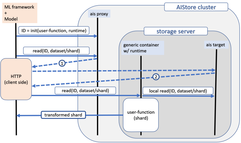
Transform

From here on, the immediate and fully expected question is: transformation. Namely – whether it’d be possible to transform datasets – not just copy but also apply a user-defined transformation to the source that may be (currently) stored in the AIS cluster, or maybe not or not entirely.

Something like:

$ ais etl init spec --name=my-custom-transform --from-file=my-custom-transform.yaml

followed by:

$ ais etl bucket my-custom-transform s3://src gs://dst --progress --refresh 3 --all

The first step deploys user containers on each clustered node. More precisely, the init-spec API call is broadcast to all target nodes; in response, each node calls K8s API to pull the corresponding image and run it locally and in parallel – but only if the container in question is not already previously deployed.

(And yes, ETL is the only aistore feature that does require Kubernetes.)

Another flavor of ais etl init command is ais etl init code – see --help for details.

That was the first step – the second is virtually identical to copying (see previous section). It’ll read remote dataset from Amazon S3, transform it, and place the result into another (e.g., Google) cloud.

As a quick aside, anything that aistore reads or writes remotely it also stores. Storing is always done in full accordance with the configured redundancy and other applicable bucket policies and – secondly – all subsequent access to the same content (that previously was remote) gets terminated inside the cluster.

Despite node and drive failures

The scripts above periodically fail and recover nodes and disks. But we could also go ahead and replace ais cp command with its ais etl counterpart – that is, replace dataset replication with dataset (offline) transformation, while leaving everything else intact.

We could do even more – select any startable job:

$ ais start <TAB-TAB>
prefetch           dsort              etl                cleanup            mirror             warm-up-metadata   move-bck
download           lru                rebalance          resilver           ec-encode          copy-bck

and run it while simultaneously taking out nodes and disks. It’ll run and, given enough redundancy in the system, it’ll recover and will keep going.

NOTE:

The ability to recover is much more fundamental than any specific job kind that’s already supported today or will be added in the future.

Not every job is startable. In fact, majority of the supported jobs have their own dedicated API and CLI, and there are still other jobs that run only on demand.

The Upshot

The beauty of copying is in the eye of the beholder. But personally, big part of it is that there’s no need to have a client. Not that clients are bad, I’m not saying that (in fact, the opposite may be true). But there’s a certain elegance and power in running self-contained jobs that are autonomously driven by the cluster and execute at (N * disk-bandwidth) aggregated throughput, where N is the total number of clustered disks.

At the core of it, there’s the (core) process whereby all nodes, in parallel, run reading and writing threads on a per (local) disk basis, each reading thread traversing local, or soon-to-be local, part of the source dataset. Whether it’d be vanilla copying or user-defined offline transformation on steroids, the underlying iterative picture is always the same:

  1. read the next object using a built-in (local or remote) or etl container-provided reader
  2. write it using built-in (local or remote), or container-provided writer
  3. repeat

Parallelism and autonomy always go hand in hand. In aistore, location rules are cluster-wide universal. Given identical (versioned, protected, and replicated) cluster map and its own disposition of local disks, each node independently decides what to read and where to write it. There’s no stepping-over, no duplication, and no conflicts.

Question to maybe take offline: how to do the “nexting” when the source is remote (i.e., not present)? How to iterate a remote source without loss of parallelism?

And so, even though it ultimately boils down to iteratively calling read and write primitives, the core process appears to be infinitely flexible in its applications.

And that’s the upshot.

References

Integrated Storage Stack for Training, Inference, and Transformations

The Problem

In the end, the choice, like the majority of important choices, comes down to a binary: either this or that. Either you go to storage, or you don’t. Either you cache a dataset in question (and then try to operate on the cache), or make the storage itself do the “operating.”

That’s binary, and that’s the bottom line.

Of course, I’m talking about ETL workloads. Machine learning has three, and only three, distinct workloads that are known at the time of this writing. And ETL is the number one.

[ Full disclosure: the other two include model training and hyperparameter optimization ]

ETL – or you can simply say “data preprocessing” because that’s what it is (my advice, though, if I may, would be to say “ETL” as it may help institute a sense of shared values, etc.) – in short, ETL is something that is usually done prior to training.

Examples? Well, ask a random person to name a fruit, and you’ll promptly hear back “an apple.” Similarly, ask anyone to name an ETL workload, and many, maybe most, will immediately respond with “augmentation”. Which in and of itself is a shortcut for a bunch of concrete sprightly verbs: flip, rotate, scale, crop, and more.

My point? My point is, and always will be, that any model – and any deep-learning neural network, in particular – is only as good as the data you feed into it. That’s why they flip and rotate and what-not. And that’s precisely why they augment or, more specifically, extract-transform-load, raw datasets commonly used to train deep learning classifiers. Preprocess, train, and repeat. Reprocess, retrain, and compare the resulting mAP (for instance). And so on.

Moreover, deep-learning over large datasets features the proverbial 3 V’s, 4 V’s, and some will even say 5 V’s, of the Big Data. That’s a lot of V’s, by the way! Popular examples include YouTube-8M, YouTube-100M, and HowTo100M. Many more examples are also named here and here.

Very few companies can routinely compute over those (yes, extremely popular) datasets. In US, you can count them all on the fingers of one hand. They all use proprietary wherewithal. In other words, there’s a problem that exists, is singularly challenging and, for all intents and purposes, unresolved.

After all, a 100 million YouTube videos is a 100 million YouTube videos – you cannot bring them all over to your machine. You cannot easily replicate 100 million YouTube videos.

And finally – before you ask – about caching. The usual, well-respected and time-honored, approach to cache the most frequently (recently) used subset of a dataset won’t work. There’s no such thing as “the most” – every single image and every second of every single video is equally and randomly accessed by a model-in-training.

Which circles me all the way back to where I’d started: the choice. The answer at this point appears to be intuitive: storage system must operate in place and in parallel. In particular, it must run user-defined ETLs on (and by) the cluster itself.

AIS

AIStore (or AIS) is a reliable distributed storage solution that can be deployed on any commodity hardware, can run user containers and functions to transform datasets inline (on the fly) and offline, scales linearly with no limitations.

AIStore is not gen-purpose storage. Rather, it is a fully-reliable extremely-lightweight object store designed from the ground up to serve as a foundation for an integrated hyper-converged stack with a focus on deep learning.

In the 3+ years the system has been in development, it has accumulated a long list of features and capabilities, all duly noted via release notes on the corresponding GitHub pages. At this stage AIS meets most common expectations in re usability, manageability, and data protection.

AIS is an elastic cluster that grows and shrinks with no downtime and can be easily-and-quickly deployed, with or without Kubernetes, anywhere from a single machine to a bare-metal cluster of any size. For Kubernetes-based deployments, there’s a whole separate repository that contains AIS deployment playbooks, Helm charts, and Kubernetes Operator.

The system features data protection and self-healing capabilities that users come to normally expect nowadays. But it can also be used as fast ad-hoc cache in front of the five (so far) supported backends, with AIS itself being the number six.

The picture below illustrates inline transformation, whereby each shard from a given distributed dataset gets transformed in-place by a user-provided function. It goes as follows:

  1. A user initiates custom transformation by executing documented REST APIs and providing either a docker image (that we can pull) or a transforming function that we further run using one of the pre-built runtimes;
  2. The API call triggers simultaneous deployment of multiple ETL containers (i.e., K8s pods) across the entire cluster: one container alongside each AIS target;
  3. Client-side application (e.g., PyTorch or TensorFlow-based training model) starts randomly reading sharded samples from a given dataset;
  4. Each read request:
    • quickly bounces off via HTTP redirect – first, of an AIS proxy (gateway) and, second, of AIS target – reaching its designated destination – the ETL container that happens to be “local” to the requested shard, after which:
    • the container performs local reading of the shard, applies user-provided transforming function to the latter, and, finally, responds inline to the original read request with the transformed bytes.

Supported

The sequence above is one of the many supported permutations that also include:

  • User-defined transformation via:
    • ETL container that runs HTTP server and implements one of the supported APIs, or
    • user function that we run ourselves given one of the supported runtimes;
  • AIS target <=> ETL container communication via:
    • HTTP redirect – as shown in the picture, or
    • AIS target performing the read and “pushing” read bytes into locally deployed ETL to further get back transformed bytes and respond to the original request.

And more. Offline – input dataset => output dataset – transformation is also available. A reverse-proxy option is supported as well, although not recommended.

Remark

In the end, the choice, like so many important choices we make, is binary. But it is good to know what can be done and what’s already actually working.

References

High performance I/O for large scale deep learning

Abstract – Training deep learning (DL) models on petascale datasets is essential for achieving competitive and state-of-the-art performance in applications such as speech, video analytics, and object recognition. However, existing distributed filesystems were not developed for the access patterns and usability requirements of DL jobs. In this paper, we describe AIStore, a highly scalable, easy-to-deploy […]

Hyperconvergence: the Litmus Test

What’s in the name

It is difficult to say when exactly the “hyper” prefix was the first time attached to “converged” infrastructure. Hyper-convergence, also known as hyperconvergence, ultimately means a fairly simple thing: running user VMs on virtualized and clustered storage appliances. The latter in turn collaborate behind the scenes to a) pool combined local storage resources to further b) share the resulting storage pool between all (or some) VMs and c) scale-out the VM’s generated workload.

That’s the definition, with an emphasis on storage. A bit of a mouthful but ultimately simple if one just pays attention to a) and b) and c) above. Players in the space include Nutanix, SimpliVity and a few other companies on one hand, and VMware on another.

Virtualized storage appliance that does storage pooling, sharing and scaling is a piece of software, often dubbed “storage controller” that is often (but not always) packaged as a separate VM on each clustered hypervisor. Inquisitive reader will note that, unlike Nutanix et al, VMware’s VSAN is part and parcel of the ESXi’s own operating system, an observation that only reinforces the point or rather the question, which is:

True Scale-Out

True scale-out always has been and will likely remain the top challenge. What’s a “true scale-out” – as opposed to limited scale-out or apparent scale-out? Well, true scale-out is the capability to scale close to linearly under all workloads. In other words, it’s the unconditional capability to scale: add new node to an existing cluster of N nodes, and you are supposed to run approximately (N + 1)/N faster. Workloads must not even be mentioned with respect to the scale-out capabilities, and if they are, there must be no fine print..

Needless to say, developers myself including will use every trick in the book and beyond, to first and foremost optimize workloads that represent (at the time of development) one or two or a few major use cases. Many of those tricks and techniques are known for decades and generally relate to the art (or rather, the craft) of building distributed storage systems.

(Note: speaking of distributed storage systems, a big and out-of-scope topic in and of itself, I will cover some of the aspects in presentation for the upcoming SNIA SDC 2015 and will post the link here, with maybe some excerpts as well)

But there’s one point, one difference that places hyperconverged clusters apart from the distributed storage legacy: locality of the clients. With advent of hyperconverged solutions and products the term local acquired a whole new dimension, simply due to the fact that those VMs that generate user traffic – each and every one of them runs locally as far as (almost) exactly 1/Nth of the storage resources.

Conceptually in that sense, clustered volatile and persistent memories are stacked as follows, with the top tier represented by local hypervisor’s RAM and the lowest tier – remote hard drives.

hyperconverged

(Note: within local-rack vs. inter-rack tiering, as well as, for instance, utilizing remote RAM to store copies or stripes of hot data, and a few other possible tiering designations are intentionally simplified out as sophisticated and not very typical today)

Adding a new node to hyperconverged cluster and placing a new bunch of VMs on it may appear to scale if much of the new I/O traffic remains local to this new node, utilizing its new RAM, its new drives and its new CPUs. De-staging (the picture above) would typically/optimally translate as gradual propagation of copies of aggregated and compressed fairly large in size logical blocks across conceptual layers, with neighboring node’s SSDs utilized first..

But then again, we’d be talking about an apparent and limited scale-out that performs marginally better but costs inevitably much more, CapEx and OpEx wise, than any run-of-the-mill virtual cluster.

Local Squared

Great number, likely a substantial majority of existing apps keep using legacy non-clustered filesystems and databases that utilize non-shared LUNs. When deploying those apps inside VMs, system administrators simply provision one, two, several vdisks/vmdks for exclusive (read: local, non-shared) usage by the VM itself.

Here again the aforementioned aspect of hyperconvergent locality comes out in force: a vendor will make double sure to keep at least caching and write-logging “parts” of those vdisks very local to the hypervisor that runs the corresponding VM. Rest assured, best of the vendors will apply the same “local-first” policy to the clustered metadata as well..

Scenarios: probabilistic, administrative and cumulative

The idea therefore is to come up with workloads that break (the indeed, highly motivated) locality of generated I/Os by forcing local hypervisor to write (to) and read from remote nodes. And not in a deferred way but inline, as part of the actual (application I/O persistent storage) datapath with client that issued the I/Os waiting for completions on the other side of the I/O pipeline..

An immediate methodological question would be: Why? Why do we need do run some abstracted workload that may in no way be similar to one produced by the intended apps? There are at least 3 answers to this one that I’ll denote as, say, probabilistic, administrative and cumulative.

Real-life workloads are probabilistic in nature: the resulting throughput, latencies and IOPS are distributed around their respective averages in complex ways which, outside pristine lab environments, is very difficult to extrapolate with bell curves. Most of the time a said workload may actively be utilizing a rather small percentage of total clustered capacity (the term for this is “working set” – a portion of total data accessed by the app at any given time). Most of the time – but not all the time: one typical issue for users and administrators is that a variety of out-of-bounds situations requires many hours, days or even weeks of continuous operation to present itself. Other examples include bursts of writes or reads (or both) that are two or more times longer than a typical burst, etc.

Administrative maintenance operations do further exacerbate. For example, deletion of older VM images that must happen from time to time on any virtualized infrastructure – when this seemingly innocuous procedure is carried out concurrently with user traffic, long-time cold data and metadata sprawled across the entire cluster suddenly comes into play – in force.

Cumulative-type complications further include fragmentation of logical and physical storage spaces that is inevitable after multiple delete and rewrite operations (of the user data, snapshots, and user VMs), as well as gradual accumulation of sector errors. This in turn will gradually increase ratios of one or two or may be both of the otherwise unlikely scenarios: random access when reading and writing sequential data, and read-modify-writes of the metadata responsible to track the fragmented “holes”.

Related to the above would be the compression+rewrite scenario: compression of aggregated sequentially written logical blocks whereby the application updates, possibly sequentially as well, its (application-level) smaller-size blocks thus forcing storage subsystem to read-modify-write (or more exactly, read-decompress-modify-compress and finally write) yet again.

Critical Litmus Test: 3 simple guidelines

The question therefore is, how to quickly exercise the most critical parts of the storage subsystem for true scale-out capability. Long and short of it boils down to the following simple rules:

1. Block size

The block size must be small, preferably 4K or 8K. The cluster that scales under application-generated small blocks will likely scale under medium (32K to 64K, some say 128K) and large blocks (1M and beyond) as well. On the other hand, a failure to scale under small blocks will likely manifest future problems in handling some or all of the scenarios mentioned above (and some that are not mentioned as well).

On the third hand, a demonstrated scale-out capability to operate on medium and large blocks does not reflect on the chances to handle tougher scenarios – in fact, there’d be no correlation whatsoever.

2. Working set

The working set must be set to at least 60% of the total clustered capacity, and at least 5 times greater than RAM of any given node. That is, the MAX(60% of total, 5x RAM).

Reason for this is that it is important to exercise the cluster under workloads that explicitly prevent “localizations” of their respective working sets.

3. I/O profile

Finally, random asynchronous I/Os with 100%, 80/20% and 50/50% of write/read ratios respectively, carrying pseudo-random payload that is either not compressible at all or compressible at or below 1.6 ratio.

That’ll do it, in combination with vdbench or any other popular micro-benchmark capable to generate pedal-to-the-metal type load that follows these 3 simple rules. Make sure not to bottleneck on CPUs and/or network links of course, and run it for at least couple hours on at least two clustered sizes, one representing a scaled-out version of the other..

Final Remarks

Stating maybe the obvious now – when benchmarking, it is important to compare apples-to-apples: same vendor, same hardware, same software, same workload scaled out proportionally – two different clustered sizes, e.g. 3 nodes and 6 nodes, for starters.

The simple fact that a given hyperconverged hardware utilizes latest-greatest SSDs may contribute to the performance that will look very good, in isolation. In comparison and under stress (above) – maybe not so much.

One way to view the current crop of hyperconverged products: a fusion of distributed storage, on one hand and hybrid/tiered storage, on another. This “fusion” is always custom, often ingenious, with tiering hidden inside to help deliver performance and assist (put it this way) scaling out..