
When training a neural network, it is not uncommon to have to run through millions of samples, with each training sample (Xi, Yi) separately obtained by a (separate) evaluation of a system function F that maps ℜn ⇒ ℜ1 and that, when given an input Xi, produces an output Yi.
Therein lies the problem: evaluations are costly. Or – slow, which also means costly and includes a variety of times: time to evaluate the function Y=F(X), time to train the network, time to keep not using the trained network while the system is running, etc.
Let’s say, there’s a system that must be learned and that is already running. Our goal would be to start optimizing early, without waiting for a fully developed, trained-and-trusted model. Would that even be possible?
Furthermore, what if the system is highly dimensional, stateful, non-linear (as far as its multi-dimensional input), and noisy (as far as its observed and measured output). The goal would be to optimize the system’s runtime behavior via controlled actions after having observed only a few, or a few hundred, (Xi, Yi) pairs. The fewer, the better.
The Idea
In short, it’s a gradient ascent via multiple neural networks. The steps are:
- First, diversify the networks so that each one ends up with its own unique training “trajectory”.
- Second, train the networks, using (and reusing) the same (X, Y) dataset of training samples.
- In parallel, exploit each of the networks to execute gradient ascents from the current local maximums of its network “siblings”.
As the term suggests, gradient ascent utilizes gradient vectors to ascend – all the way up to the function’s maximum. Since maximizing F(X) is the same as minimizing -F(X), the only thing that matters is the subject of optimization: the system’s own output versus, for instance, a distance from the corresponding function F, which is a function in its own right, often called a cost or, interchangeably, a loss.
In our case, we’d want both – concurrently. But first and foremost, we want the global max F.
The Logic
The essential logic goes as follows:
 The statements 1 through 3 construct the specified number of neural networks (NNs) and their respective “runners” – the entities that asynchronously and concurrently execute NN training cycles. Network “diversity” (at 2) is achieved via hyperparameters and network architectures. In the benchmark (next section) I’ve also used a variety of optimization algorithms (namely Rprop, ADAM, RMSprop), and random zeroing-out of the weight matrices as per the specified sparsity.
At 4, we pretrain the networks on a first portion of the common training pool. At 6, we execute the main loop that consists of 3 nested loops, with the innermost 6.1.1.1 and 6.1.1.2 generating new training samples, incrementing numevals counter, and expanding the pool.
That’s about it. There are risks though, and pitfalls. Since partially trained networks generate gradients that can only be partially “trusted,” the risks involve mispartitioning of the evaluation budget between the pretraining phase at 4 and the main loop at 6. This can be dealt with by gradually increasing (multiplicatively decreasing) the number of gradient “steps,” and monitoring the success.
There’s also a general lack of convexity of the underlying system, manifesting itself in runners getting stuck in their respective local maximums. Imagine a system with 3 local maximums and 30 properly randomized neural networks – what would be the chances of all 30 getting stuck on the left and/or the right sides of the picture:

What would be the chances for k >> m, where k is the number of random networks, m – the number of local maximums?..
The Benchmark
A simplified and reduced Golang implementation of the above can be found on my github. Here, all NN runners execute their respective goroutines using their own fixed-size training “windows” into a common stream of training samples. The (simplified) division of responsibilities is as follows: runners operate on their respective windows, centralized logic rotates the windows counterclockwise when the time is right. In effect, each runner “sees,” and takes advantage of, every single evaluation, in parallel.
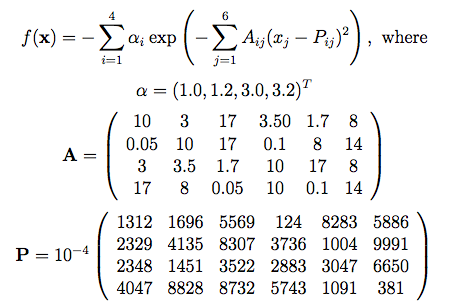
A number of synthetic benchmarks is available and widely used to compare global optimization methods. This includes Hartmann-6 featuring multiple local optima in a 6-dimensional unit hypercube. For the numbers of concurrent networks varying between 1 and 30, the resulting picture looks as follows:

The vertical axis on this 3-dimensional chart represents the distance from the global maximum (smaller is better), the horizontal axis – Hartmann-6 calls (from 300 to 2300), the “depth” axis – number of neural networks. The worst result is for the {k = 1} configuration consisting of a single network.
Evolution
There’s an alternative to SGD-based optimization – the so-called Natural Evolution Strategies (NES) family of the algorithms. This one comes with important benefits that allow to, for instance, fork the most “successful” or “promising” network, train it separately for a while, then merge back with its parent – the merger producing a better trained result.
The motivation remains the same: parallel training combined with global collaboration. One reason to collaborate globally boils down to finding a global maximum (as above), or – running an effective and fast multimodal (as in: good enough) optimization. In the NES case, though, collaboration gets an extra “dimension:” reusing the other network’s weights, hyperparameters, and architecture.
To be continued.
