It’s been noted before that Ceph benchmarks produce results that are lower than expected. Take for instance the most recent FAST’16 [BTrDB] paper (quote):
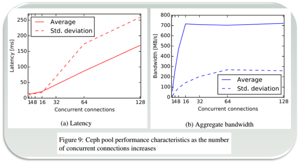
<snip> Applying this backpressure early prevents Ceph from reaching pathological latencies. Consider Figure 9a where it is apparent that not only does the Ceph operation latency increase with the number of concurrent write operations, but it develops a long fat tail, with the standard deviation exceeding the mean. Furthermore, this latency buys nothing, as Figure 9b shows that the aggregate bandwidth plateaus…

The above is indeed a textbook case (courtesy of [BTrBD]) of fat-tailed distribution, the one that deviates from its mean with high probability having either undefined or unbounded standard deviation (sigma). But wait.. the fat-tailed latency problem is by no means Ceph-specific.
Disclaimer:
Nexenta produces a competing solution that is called NexentaEdge. Secondly, needless to say that opinions expressed in this text are strictly and solely my own.
There are multiple reasons to single-out Ceph, the most researched and likely the most widely used general-purpose distributed storage stack. Ceph is an open source project as well, open for in-depth reviews. CRUSH remains one of the best content distribution algorithms. In sum, Ceph is as close as it gets to being a representative of the current generation – generation of post-Dynamo distributed storage systems.
The problem though affects majority of fully-distributed storage systems. To add insult to injury, it cannot be easily bug-fixed. The fat-tailed, heavy-tailed, long-tailed latency problem is in fact the other side of the uniformly-distributed “coin”.
The Conflict
A distributed storage cluster consists of multiple user-facing Storage Initiators (henceforth, “initiators”) and multiple reading/writing Storage Targets (“targets”).
Both initiators and targets execute concurrently and in parallel, the former – app requests, the latter – disk I/Os. Often {initiator + target} pairs are bundled as dual-function daemons within their respective clustered nodes – case in point (hyper)converged architectures, but not only.
The defining characteristic of a fully distributed cluster is that the path from an initiator to a target is direct. The datapath does not “cross” any central authority.
There is a lot of varying intelligence typically built into existing initiators, to help them decide where and how to route I/O requests. This intelligence, however, executes in the management and control (error processing) planes leaving fast path data distribution decisions totally up to the clustered frontend – to a given storage initiator.
This is exactly why do we have the following generic conflict – in Ceph, and in Swift, and in others.

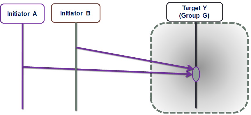
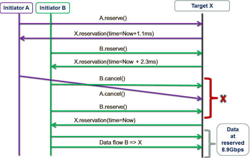
Figure 1. The Conflict
The figure depicts initiators A and B simultaneously reaching out to the same target Y. Since there’s no metadata server (MDS), centralized arbiter/load-balancer or any other kind of central logic in the datapath, each initiator simply goes ahead and reaches out based on the best information it had at the time.
From the target Y’s perspective, however, it just happened so that the two requests arrive in rapid succession within the same interval – the interval that, on average, corresponds to a single I/O request under a given workload (aka inter-arrival time).
Visualize a storage cluster consisting of identical nodes, where user data is uniformly distributed by multiple initiators, thus providing, on average, well-balanced resource utilization: CPU, network, I/O bandwidth and disk capacity of individual targets. Here’s the pertinent question: what is the probability of a conflict depicted above, where storage targets are forced to handle multiple requests within a single interval of time.
Poisson approximation
In statistics, a Poisson experiment must have the following defining properties:
- The experiment results in outcomes that can be classified as successes or failures.
- The average number of successes that occurs in a specified time interval is known.
- The probability that a success will occur is proportional to the size of the interval.
- The probability that a success will occur in an extremely small interval is virtually zero.
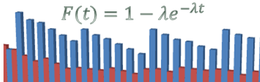
To make the connection, I’ll go out on a limb and say this: a very large fully distributed storage cluster under a fully random workload and sufficiently large working set can be (***) approximated as a massive Poisson experiment-generating machine. Whereby the target’s chances to see two or more I/O requests during a time interval t would compute as: Therefore, at a sustained workload of, say, modest 10K per-target IOPS, the average inter-I/O interval would be 100μs. Given uniform distribution of I/O requests, the probability of two or more requests within this average 100μs interval is precisely:
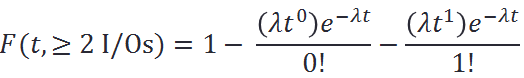
 Meaning, for at least a quarter of all 100μs long intervals each target should expect to handle at least 2 interval-sharing requests. And in about 2% of all time the number spikes up to 4 or more, as per:
Since storage clusters normally run many hours, days and months at a time, the 2% must be understood as accumulated minutes and hours of random 4x spikes.
Uniform distributions fair well when the cluster is – on average – underutilized. But if and when the load and pressure grows beyond 50% utilization and the resulting average per-I/O interval shrinks proportionally, then very quickly and quite frequently the targets are required to execute well above the average, and ultimately beyond their provisioned maximum bandwidth.
How frequently? At 50% utilization each clustered target must be expected to run at least 2 times faster than its own maximum performance at least 2% of the time. That is, assuming of course that the entire storage system can be modeled as a Poisson process.
But can it?
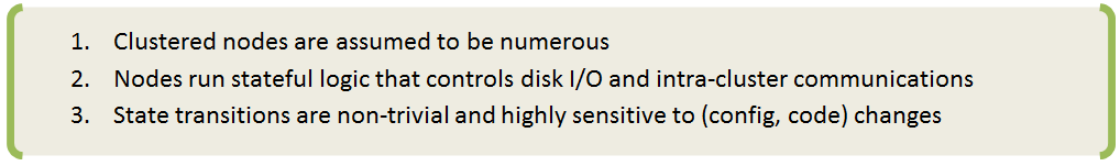
(***) Poisson processes are memoryless and, simultaneously, stateless – the two fine and abstract properties that are definitely not present in any real-life storage situation, distributed or local. Things get cached and journaled, aggregated and deduplicated. Generally, storage nodes (like the ones shown on Fig. 1) at any point in time have a wealth of accumulated state to deal with.
There are also multiple ways by which the targets may share their feedback and their own state with initiators, and each of these “ways” would create an additional state in the corresponding cluster-representing Markov’s chain which ultimately can become rather huge and unwieldy..
My sense though is (and here I’m frankly on shaky grounds) that given the (a, b, c, d) assumptions below, the Poisson approximation is valid and does hold.
(a) large fully distributed storage cluster;
(b) random workload;
(c) massive working set that tramples any and every attempt to cache;
(d) direct and uniform initiator ⇒ target distribution of data.
At the very least it gives an idea.
Synthetic Idea
To recap:
- Distributed clustering whereby a certain segment of datapath and/or metadata path is centralized – is a legacy that does not scale;
- Total decentralization of both data and metadata I/O processing via uniform and direct initiator-to-target distribution is the characterizing property of modern-time storage architectures. It works great but only under low to medium utilizations.
The idea is to inject a bit of centralization into the otherwise fully and uniformly distributed cluster, to provide for scale and, simultaneously, true balance under stress. An example of one such protocol follows, along with benchmarks and comparison in the second (and separate) part of this text.
On the Go
The implementation involves homegrown SURGE framework that is written in Go. I’m using Go mostly due to its built-in goroutines and channels – the language primitives that were invented to quickly write pieces of communicating logic that independently and concurrently run inside distributed “nodes”. As many nodes as your heart desires..
In SURGE each storage node (initiator or target) is a separate lightweight thread: a goroutine. The framework connects all configured nodes bi-directionally, via a pair of per node (Tx, Rx) Go channels. At model’s startup all clustered nodes (of this model) get automatically connected and ready to Go: send, receive and handle events and I/O requests from all other nodes.
There are various infrastructure classes (aka types) and utilities reused by the previously implemented models, for instance a rate bucket type that helps implement network and disk bandwidth limitations, and many more (see for instance the entry on this site titled Choosy Initiator).
Each SURGE model is an event-distributing event-driven machine. Quoting one previous text on this site:
Everything that happens in a modeled world is a result of prior events, and the result of everything-that-happens is: new events. Event timings define the progression of Time itself..
Clustered configuration is practically unlimited. Each data frame and each control packet is a separate timed event over a separate peer-to-peer channel. The number of events exchanged during a single given benchmark is, frankly, mind-blowing – it blows my mind, it still does.
Load Balancing Groups with group leaders
The new model (main piece of the source code here) represents a storage cluster that consists of load balancing groups of storage targets. Group size is configurable, with the only guideline that it corresponds to the required redundancy – due to the fact that each group acts as a whole as far as storing/retrieving redundant content.
The protocol leverages multicast replication of user data, and control plane that is, at least in part, terminated by a per-group selected leader, aka Group Proxy (from here on simply: proxy). In the simulation a proxy is a storage target with a minimal ID inside its own group.
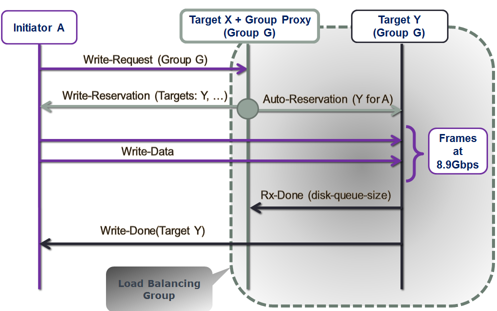
Let’s see how it works without going yet into much detail – picture below illustrates the write/put sequence:
Figure 2. Write Sequence
- initiator A sends write request to the target X, which is also (in its second role) – a group leader or a proxy responsible(*) for its group G;
- target X then performs a certain non-trivial computation based on outstanding previous requests – from all initiators;
- this results in two back-to-back transactions from/by the target X:
- write reservation sent to the initiator A, and
- auto-reservations sent to the selected targets in the group G, made on behalf of those selected targets (note that target X depicted here includes itself into the selection process);
- given the reservation time window and the list of selected targets, initiator A then multicasts data –one data frame at a time, at provisioned link bandwidth (which is configurable, with control bandwidth and overhead factored-in);
- once the entire payload is received, each of the selected targets updates proxy X with its current size of its disk queue;
- finally, when the payload is safely stored, each selected target sends an ACK to the initiator A indicating: done.
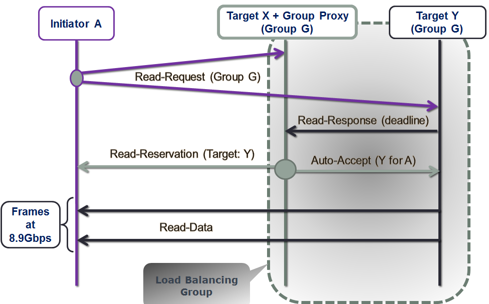
As far as read/get, the pipeline starts with the read request delivered to all members of the group (Fig. 3). The idea is the same though: it is up to the proxy to decide who’s handling the read. More exactly:
Figure 3. Read Sequence
- initiator A maps or hashes the read (or rather name of the file, ID of the chunk, LBA of the block, etc.) onto a group G, and then sends the request to all members of this same G;
- target X which happens to be the group leader (or, proxy) receives read responses from those targets in the group that store the corresponding data;
- once target X collects all or some(*) responses, it makes an educated decision. Similar to the write case (Fig. 2), this decision involves looking at all previous-but-still-outstanding I/O requests, and computing the best target to perform the read;
- finally, selected target sends the data back to the requesting initiator, which prior to this point would have been already updated with its (the target’s) ID and the time (deadline) to expect the read to commence.
Notice that in both read and write cases it is the group proxy that performs behind-the-scenes tracking of who-does-what-when for the entire group. The proxy, effectively, is listening on everything transpiring on the group-targeting control plane, and makes inline I/O routing decisions on behalf of the rest of group members.
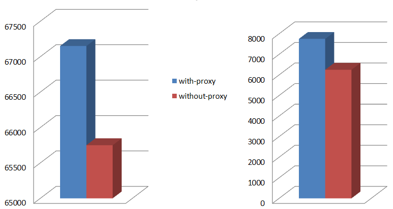
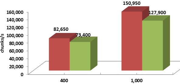
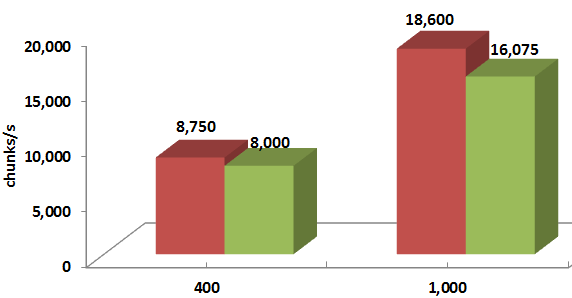
Instead of conclusions
Wrapping up: one quick summary chart that shows the respective with group proxy and without group proxy benchmark-average performances expressed as chunks-per-second. The 50% read, 50% write workload is directed into 90 simulated targets by as many initiators, and the chunk sizes are 128K on the left, and 1M on the right, respectively:

Figure 4. Average throughput
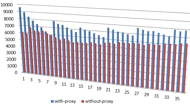
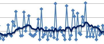
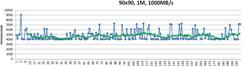
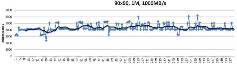
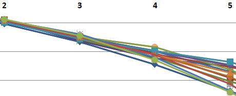
And here’s the throughput over time, for the same 50%/50% workload and 1MB chunk size:

Figure 5. Throughput for 1M chunk
This experiment corresponds to the 1ae1388 commit. In the second upcoming part of the series I’ll try to show how exactly the comparison is done, and why exactly the results are what they are.
Evolution, some say, moves is spiraling circles and cycles. Software paradigms evolve and mutate, with every other iteration reintroducing stuff that was buried deep in the past. Or so it seems.
Post-Dynamo clusters that have evolved in forms of distributed block arrays, object storage clusters and NoSQL databases, reject any centralized processing in the datapath. There is a multifaceted set of interesting limitations that comes with that. What could be the better protocol? To be continued…
 None of this is uncommon. For one thing, we live at a time of ever-exploding problem sizes. Bigger problems lead to bigger clusters with nodes that, when failed, get replaced wholesale.