
What is data storage? Dictionaries define data as information, and storage as “act of storing” or “space for storing.” A data storage system, then, is something that stores, keeps, protects, and ultimately conserves information. When we talk about data storage, we must therefore consider conservation and the laws of thereof.
The conservation laws are the most fundamental, the most universal, the most principle of all the laws of nature. Physical systems conserve momentum and energy. Quantum mechanical systems additionally conserve information. A quantum mechanical system manages to conserve its information even in the most extreme conditions, such as the immediate proximity of a gigantic black hole (see Black hole information paradox and ER = EPR, in that sequence).
Moreover, all physical systems abide by their system-specific laws of motion. Electromagnetic systems abide by the electromagnetic laws of motion, thermodynamic systems – by thermodynamic, and so on. Newton’s second law of motion (circa 1687), the Second law of thermodynamics, the Maxwell-Faraday equation, the Schrödinger wavefunction, the Einstein field equations – these are various laws of motion expressed as differential equations.
At this point, I’m going to go on a limb and posit that a storage system is a physical system. Further, a good storage system is a quantum mechanical system that preserves information with respect to its “motions” that include:
- relocation, replication, rebalancing
- snapshotting, cloning
- compression, encryption, deduplication
- decompression, decryption, un-snapshotting
and more.
In layman terms, the goodness of a storage system is henceforth defined as its compliance with the universal conservation laws and its ability to behave like any other well-behaved physical system. But what does it mean “to behave”? Well, it means to move, transform and evolve according to the system-specific laws of motion. The laws of motion, in turn, abide by the conservation laws, while those, in their most general presentation, state that some quantity Z in the mathematical description of a system’s evolution must remain constant. In effect, Z must remain invariant. Let’s talk therefore about:
Invariance and symmetry
The conservation laws are, what many scientists call, “principle laws” – universal laws about other universal laws (see The Unity Of The Universe by David Deutsch, at 10:35). It’s the conservation laws that define universal laws of motion, and not the other way around. In the hierarchy of all laws, the conservation laws are strategically positioned at the base.
A word on the established terminology. In the scientific description of conservation laws, the terms “symmetry” and “invariance” are interchangeable, with “symmetry” implying a specific class, a family, or better yet, a group of transformations. The following two statements are equivalent and should make this last point very clear:
(1) A conservation law states that a particular measurable property of a system does not change as the system evolves. (2) A conservation law states that a particular measurable property of a system remains invariant with respect to certain transformations that in combination constitute a symmetry (group).
Similarly, a good storage system (that conserves information in presence of lossless stateful transformations) is symmetric with respect to those transformations (aka translations).
But which transformations constitute a good-storage-system’s symmetry group? The answer will be based on yet another universal law that states:
What’s not forbidden is allowed. Moreover, everything that is not forbidden is compulsory.
For a good storage system, the direct and unavoidable implication of the above is that the system must support all stateful transitions resulting from the not forbidden (or rather, not yet forbidden) compressions, encryptions, replications, deduplications and so on.
Q.E.D.
So far, I’ve laid the groundwork to introduce the main topic: a perfect storage system. This is a good system of unimpeachable integrity abiding by the universal conservation laws, the most fundamental of which is that information is never lost. The storage system that evolves without ever taxing the user for its internal evolution.
That’s the perfection we’ll be looking for in the subsequent sections.
The Plan
One useful approach to build something new is to first destroy the current version that is getting old (or deemed to be old by a recent college grad). And then to think about the next step. This process is called creative destruction (with an emphasis on “creative”) and implies a certain reuse rather than total uncompromising annihilation. The typical roadmap is:
- Blow the old version to smithereens, while setting aside a couple of original building blocks;
- Refashion those creatively, and then immediately proceed to build the new.
But what about the building blocks? Which ones shall we select, retain and, subsequently, refashion? That is the question, and the sole purpose of this text, which also entails:
- Introductory insight into the crucial value of intuition in storage engineering – in the Section “Trust your intuition”;
- Historical and literary allusions – in Sections “1982” and “Down the rabbit hole”;
- Creative destruction (with an emphasis on “destruction”) of contemporary art – in “Genericity” and “Reductionism”;
- Forewarning of unexpected dangers that are to be expected – in “Against corruption”;
- A note on natural selection in storage – in “Darwinism.”
You can also TLDR directly to the namesake Section – therein lies an important clue on how to start building a perfect storage system.
Trust your intuition
You are a software architect. One day you start early, work for a while, and devise a data structure. It is now sitting in the corner of your screen – a bunch of pointers sticking out of it, a few carefully crafted content fields. A question arises in the back of your mind: is this it?
Lifted from the depths of the unconscious, the question is what will happen once everything is said and done, and after the bits get GA-ed, shipped, deployed as a live storage system brimming with user data: That’s the human condition – we have no ways of finding out. Visualize a shopping mall: in an infinitely long row of data structures, each one will be neatly packaged and labeled with its pros and cons. The pros will include a faster disk access for sequential I/O, for instance. (How much faster? The label won’t tell.) The cons – fragmentation that would require compaction. (Was this information helpful? Give us your feedback by checking one of the boxes.)
1982
To search for real answers, we need to go all the way back – to early frontiers.
The year is 1982. Pan Am is still operating across the Atlantic, but the 830 bombing will soon usher a new era. Recession grips the US. Brezhnev dies after 17 years of ruling the communist party and the USSR. The first CD player. Survivor’s Eye Of The Tiger. Times Man of the Year is the personal computer. A graduate student at UC Berkeley follows in the footsteps of other Unix pioneers (Bill Joy et al.), to build the very first filesystem that was later called Unix File System, or UFS.

Figure 1. UFS inode
UFS introduced the inode data structure (Fig. 1). UFS used (and keeps using) the inode to store UFS files in UFS directories.
Enough of the trivia though, and so much for a glorious history. A lot has changed in the intervening years except one little thing – the file being a byte array over a bunch of 512n, 512e, or 4Kn physical segments stitched together by the filesystem. (Nobody knows that last bit except maybe a few storage-systems engineers, and even they often forget.)
Meaning that, in all past, current and future filesystems, there’s a core metadata structure that represents and implements a file as a “sequence of bytes.” All existing and future files can be traced back to the very first inode in the Fig. 1.
That’s pretty damn remarkable.
Down the rabbit hole
You are a storage architect. One day you start early and work till dusk. You keep working into the night when the voices retreat, street sounds die out, and the darkness falls. And then – you see it: your storage system.

From a distance, it looks like a giant web splattered across non-volatile storage media that has been pooled together for greater capacity. It’s a giant mess, a jumble of trunks, branches, and leaves – growing, forking, intertwining, and multiplying.
When you get closer – in the process that must be quaintly familiar to anyone who ever experienced vertiginous Mandelbrot zooms or who used to fall with Alice down the rabbit hole – when you get closer, the cluttered tendrils become separable, and you see a picture that is eerily familiar. Oh yes, it’s a gigantic directed graph, not necessarily acyclic albeit traversable from the top down (at the top, it resembles a forest with a few discernable roots).
(Keep falling, accelerating, zooming-in.)
As the resolution magnifies, distinct nodes shift into focus, with their directed edges of different kinds. The most abundant will be the parent-contains-child type of edge, but there are others, connecting each other forward, backward, and sideways.
Gradually, a pattern emerges. You don’t notice it for a while because at first, all nodes appear to be infinitely different and categorically unique. It is only when you step back up a little bit, you start recognizing the node’s types aka metadata structures.
Some of those structures seem to be repetitive. As you stare at it some more, you realize that the word “repetitive” does not adequately describe the situation. Two, or maybe five of those metadata types cover most of the graph. They dominate the rest by a wide margin.
(And it is with this uneasy thought you wake up.)
Genericity
There are only two viable perspectives of the world: user and system. The user’s point of view is that the data is deeply structured, hierarchically layered, intricately cross-referenced, and – on top of all of the above – multimedia-rich. On-disk though, it’s a graph that is so generic that its apparent genericity gives a new meaning to being generic.
At the same time, there’s the amazing, demonstrated, and million times confirmed efficiency of storing/retrieving data in all its incredible variety by utilizing just a handful metadata types. Reducing, in effect, the entire world to a few elementary “particles” of its as-yet undiscovered standard model.

Figure 2. The Standard Model of particle physics
Reductionism
Building a storage system is excruciatingly hard. There’s one thing that’s harder, though: seeing it through – living long enough to see it through.
Can we somehow reduce the mind-blowing complexity of a storage system? My answer is Yes. But first, before reducing anything anywhere, let’s come to terms with Reductionism.
Reductionism refers to several related philosophical ideas, says Wikipedia, and goes on to touch upon each of those in the spheres of natural sciences, mathematics, religion, and philosophy.
Sadly, storage engineering is never mentioned – not by the Wikipedia, or by any other reputable source.
Let’s close that knowledge gap. First, notice that Reductionism is a meta-philosophical abstraction that, by all appearances, belongs to the highest order of the purest Platonic Forms. At the same time, Reductionism is deceptively easy to grasp intuitively. What’s not easy at all is to define it.
Let’s, therefore, go ahead and define Reductionism in a way that can be dear and near to the hearts of software engineers.
The essence of Reductionism is to impose a can-be-derived-from ordering on a given theory or body of knowledge (broadly, on any phenomenon). Accordingly, some entities, properties or substances arise or emerge out of more fundamental entities, properties, and substances, respectively. And yet, those new ones (that have arisen or emerged) are in some sense irreducible.
There are many notable examples. The entire periodic table can be step-by-step built from the Standard Model’s particles (Fig. 2 above).
Only 3 of the 17 known particles (aka quantum fields) are required to build the entirety of ordinary matter (Fig. 2). Plus, the neutrino that takes part in the process of changing the atomic nucleus into a different kind.
In Mathematics, it’ll take a certain effort to find an area or a field that’s irreducible to natural numbers. Hence, the lower part of the corresponding “reductionist” pyramid of all of Math looks as follows:
Figure 3. The pyramid of numbers
In the picture above integers can be derived from the natural numbers via subtraction, rational numbers from integers – via division, real numbers from rational numbers – via a Dedekind cut, and complex numbers from real numbers – via the pairing of real numbers and defining the multiplication rule as follows:
(a, b) * (c, d) = (ac – bd, ad + bc)
where a, b, c, d are real numbers.
The multiplication rule may seem non-obvious and not very intuitive. It becomes abundantly clear, however, once the complex numbers are expressed in polar or, better yet, exponential forms.
Maybe it’s a cliché to say that mathematics builds on itself. The same, however, applies across the board to any branch of science or technology. Very often there’ll be a tall and growing taller pyramid, with a narrow foundation and layers upon layers of the derived complexity. Something that looks as follows, for instance: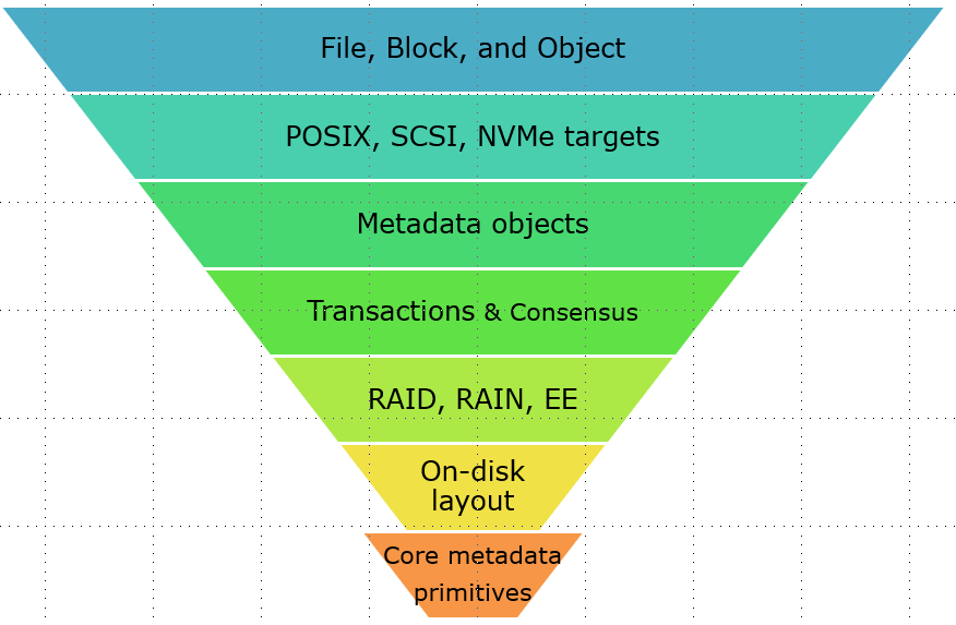
Reductionism must be equivalent to consistent build-up as it is fully based on the ability to incontrovertibly derive the complexity of the upper layers from the building blocks of the lower layers, and ultimately, from the most basic and most irreducible axioms. Without this internally-consistent continuous build-up, there’d be nothing to reduce in the first place. Instead, there would be a confounding chaos, a primordial timeless void.
Against corruption
Here’s what we know beyond any shred of doubt: on-disk layout is self-reproducing, and the amount of its self-reproduction is driven exclusively by the sheer size and granularity of the user data.
On the other hand, a storage system must retain its on-disk consistency at all times and under any circumstances. A diverse and extended set of those circumstances comprises the entire disk lore that is crammed with tales of rapidly degrading disks, disks turning read-only, disks turning themselves into bricks, and disks conspiring with other disks to turn themselves into bricks.
There’s also silent data corruption which, as the name implies, corrupts rather silently albeit indiscriminately.
In layman terms, data corruption is called silent when the storage system does report it while the underlying solid-state or hard drive doesn’t (or wouldn’t).
Some studies attribute up to 10% of catastrophic storage failures to silent corruption. Other studies observe that “SLC drives, which are targeted at the enterprise market <snip>, are not more reliable than the lower end MLC drives,” thus providing a great educational value. There is, however, not a single study of what should’ve been appropriately called a silent undetected corruption. The related statistical data is probably just too painful to document.
Finally, the software/firmware malfunction that comes on top of all of the above and, to be honest, tops it all. It manifests itself in a rich variety of assorted colorfully named conditions: phantom writes and misdirected reads, to name a few.
About Darwinism
Nature repeats itself, especially if the repetition pays off. And if not, then not – end of story, thank you very much. The same is true for storage systems – some of them, frankly, keep capturing user data as we speak. But not all, not by a long stretch.
There are also those storage systems that linger. In fact, some of them linger for so much time that you’d take them for granted, as a steady fixture of the environment. But that’s beside the point. The point is, never-ever will those systems thrive and multiply in the strict Darwinian sense that defies corruption and defines success as the total deployed capacity.
TLDR
Here’s the upshot of my so far carefully constructed argument:
- Storage systems rely on a handful of their internal (core) data structures to store just about everything;
- Generations of engineers, while firmly standing on the shoulders of the giants, augment those core data structures incrementally and anecdotally;
- Instead, when building a good storage system of the future, our focus should be directed solely at the core;
- We shall carve the perfection out of the existing raw material by applying conservation laws.
That’ll be the plan in sum and substance. To begin with, let’s consider a conventional core data structure in an existing storage system. It could be a file or a directory (metadata type) in a filesystem. It can be an object or a chunk of an object in an object store, a key or a value in a key/value store, a row, a column, or a table in a database. In short, it could be any and all of those things.
Now, visualize one such structure. If you absolutely have to have something in front of your eyes, take the inode from the Section “1982” – as good a starting point as any. Distilled to its pure essence, it will look as follows:
Figure 4. The core metadata, refined and purified
That’d be our initial building block: arbitrary content and maybe a few pointers to connect adjacent nodes: children, parents and/or siblings. Incidentally, the content is not relevant at this point (it may be later) – what’s relevant is the surrounding environment, the stage, and the World. Paraphrasing Shakespeare, all the World is a lattice, and nodes in it are… no, not actors – travelers. The nodes move around:

Figure 5. Basic transformations: a) move, b) replicate
The lattice is an n-dimensional grid (only two dimensions are shown in the Fig. 5 and elsewhere) that reflects addressing within the storage graph. Concrete storage-addressing implementations may include: keys (to address values), qualified names and offsets, volume IDs and LBAs, URIs and shard sequence numbers, and much more. To that end, our lattice/grid World is a tool to conduct thought experiments (gedankenexperiments) while abstracting out implementation specifics.
The leftmost part of the Fig. 5 depicts a snippet of the World with two nodes A and B placed in strict accordance with their respective cartesian coordinates. Simultaneously, the A would be pointing at the B via the A’s own internal Fig. 4 structure. That’s what we have – the setup at Time Zero.
What happens next? Well, what happens is that something happens, and node B moves (Fig. 5a) or replicates (Fig. 5b). The move (aka migration) could have resulted from the B getting compressed or encrypted in place. Or perhaps, getting tiered away from a dying disk. Either way, the result is a new World grid location denoted as B’. And since, excepting the change in coordinates, B’ is the same B, the picture illustrates the distinction between identity and location. The distinction that in and of itself is informative.
Many storage systems today bundle, pack, or otherwise merge identities and locations, the practice that became especially popular with wide-spread acceptance of the consistent hashing. In effect, those systems may be violating the symmetry with respect to spatial translations.
In a good storage system, the corresponding symmetry must be preserved even though it may (appear to) not directly connect to user requirements or auxiliary pragmatic considerations. In effect, the requirement of complying with the principle conservation laws changes our perspective on what is crucially important and what can maybe wait.
The long and short of this is that the most basic spatial symmetry implies a certain upgrade in the initial building block shown in the Fig. 4 above. The concrete implementation of this “upgrade” will depend on specifics and is therefore omitted.
Next, compare the following two scenarios where node B is referenced in the World grid by two other nodes: A and C.

Figure 6. Counting the references
Skipping for brevity the otherwise timely discussion of reference counting, let’s just point out that the Fig. 6a and Fig. 6b – are different. In a good storage system, the corresponding informative difference (which typically gets discarded without so much as a blink) must be preserved. This will most likely have implications for our future perfect building block.
To give one final example, consider a split and a merge – two lossless transformations that are also mutually inverse:
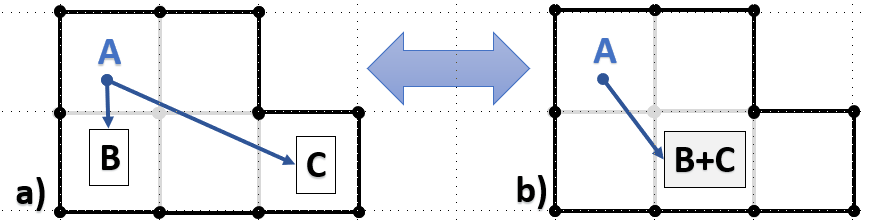
Figure 7. The logical boundaries must be flexible, subject to evolution of the system
Here again, from the user perspective, and assuming the names B and C are not externally visible, nothing really changes between the Figures 7a and 7b. On the other hand, there’s a material change that is distinctly different from the previous two gedankenexperiments. The change that must be a) permitted by the storage system, and b) preserved, information-content wise.
Further, conducting split and merge transformations en masse will likely require a larger-than-building-block abstraction: an object and its version, or maybe a dataset and its snapshot. Or even, a dataset and its immutable mutable snapshot – the snapshot that remains totally invincible in the presence of splits, merges, and other lossless transforms, members of the corresponding storage symmetry groups.
In conclusion
Storage systems that continuously evolve and self-optimize via natively supported lossless transformations? That’s maybe one idea to think about.
There’s also the crucial issue of controlling the complexity which tends to go through the roof in storage projects. Pick your own “inode” and build it up, one step at a time and block by perfect block? You decide.
Other questions and topics will have to remain out of scope. This includes immutable mutable snapshotting (IMS), ways to define it, and means to realize it. The potential role of the IMS in providing for the translational storage symmetries cannot be underestimated.


 Here’s how this formula is working out. Recall that


